9 Text mining with tidytext
This chapter is an introduction to text mining with the powerful R package tidytext.
Let’s first install the packages that we will use:
install.packages("tidytext")4
install.packages("textdata")
The package
texdatainclude useful dictionaries; the packagetidytextincludes the basic functions we will use for text mining.
library(tidyverse)
library(tidytext)
library(ggplot2)
9.1 From raw text to document term matrix
We will illustrate the basics of text analysis by first using the following set of three documents:
- Document 1: “I love love data analytics”
- Document 2: “I dislike data analytics”
- Document 3: “I love data.”
t = tibble(text = c("I love love data analytics", "I dislike data analytics","I love data."),
           document_id=c(1,2,3))
t
## # A tibble: 3 × 2
## text document_id
## <chr> <dbl>
## 1 I love love data analytics 1
## 2 I dislike data analytics 2
## 3 I love data. 39.1.1 tidytext::unnest_tokens
The package tidytext includes the function unnest_tokens. This powerful function takes as input a raw text column from our tibble, and transforms it into a new tibble where each term in the raw text becomes a row:
t1 = t %>% unnest_tokens(word, text)
t1
## # A tibble: 12 × 2
## document_id word
## <dbl> <chr>
## 1 1 i
## 2 1 love
## 3 1 love
## 4 1 data
## 5 1 analytics
## 6 2 i
## 7 2 dislike
## 8 2 data
## 9 2 analytics
## 10 3 i
## 11 3 love
## 12 3 data
The function
unnest_tokensby default converts each word to lowercase and removes punctuation.
Even though the tibble has expanded to 12 rows (i.e., a row for each word in column
textof the initial tibble), the rest of the columns of the initial tibble (i.e.,document_id) have been retained, in a way that we can still recover which word belongs to which document.
9.1.2 Stop words
Many words are used frequently and often provide little useful information. We call these words stop_words.
The tidytext package come with a stop_words dataset (list):
stop_words %>% head## # A tibble: 6 × 2
## word lexicon
## <chr> <chr>
## 1 a SMART
## 2 a's SMART
## 3 able SMART
## 4 about SMART
## 5 above SMART
## 6 according SMARTThe columnb
lexiconin the tibblestop_wordsidentifies from which lexicon a stopword is taken from. (You can find more here: https://juliasilge.github.io/tidytext/reference/stop_words.html)
Often, we want to remove such stop words from the text to reduce noise and retain only useful textual information.
Since these words are stored in a tibble, we can remove them from our documents with the verb filter and the membership operator %in%:
t1 %>% filter(!word %in% stop_words$word)## # A tibble: 9 × 2
## document_id word
## <dbl> <chr>
## 1 1 love
## 2 1 love
## 3 1 data
## 4 1 analytics
## 5 2 dislike
## 6 2 data
## 7 2 analytics
## 8 3 love
## 9 3 data9.1.3 Joins
Alternatively, we can use a function from the dplyr join family. But what is a join? In simple terms, a join is an operation that in its simplest form, it takes a left tibble and matches information for each row from a right tibble based on a common column between the two.
9.1.3.1 Inner joins
Assume that we have the following two tibbles:
join1 = tibble(id=c(1,2), info=c("some","info"))
join1
## # A tibble: 2 × 2
## id info
## <dbl> <chr>
## 1 1 some
## 2 2 infojoin2 = tibble(id=c(1,2,3), some_add_info = c("some","add","info"))
join2## # A tibble: 3 × 2
## id some_add_info
## <dbl> <chr>
## 1 1 some
## 2 2 add
## 3 3 infoThe simplest and most straightforward type of join is called inner join. This join retains only rows that are found in both tibbles. For instance, we can use an inner join to combine the two tibbles join1 and join2 based on their column column id:
join1 %>% inner_join(join2, by="id")## # A tibble: 2 × 3
## id info some_add_info
## <dbl> <chr> <chr>
## 1 1 some some
## 2 2 info add9.1.3.2 Left joins
If we want to retain all the information from one of the two tibbles, we can use a left_join, where we place the tibble we care about retaining to the left of the join:
join2 %>% left_join(join1, by="id")## # A tibble: 3 × 3
## id some_add_info info
## <dbl> <chr> <chr>
## 1 1 some some
## 2 2 add info
## 3 3 info <NA>
Note that the left join fills elements of the final tibble that are not found in both tibbles with NAs
9.1.3.3 Anti joins
Now, a different type of join is called anti_join. This type of join retains only the rows of the tibble that is placed to the left of the join that are not found in the tibble that is placed to the right. For instance:
join2 %>% anti_join(join1, by="id")## # A tibble: 1 × 2
## id some_add_info
## <dbl> <chr>
## 1 3 info9.1.3.4 Anti join stop words
Back to our example, an alternative way of removing stop words would be to use an anti_join between the stop_words tibble and our main tibble:
t1 %>% anti_join(stop_words, by="word")## # A tibble: 9 × 2
## document_id word
## <dbl> <chr>
## 1 1 love
## 2 1 love
## 3 1 data
## 4 1 analytics
## 5 2 dislike
## 6 2 data
## 7 2 analytics
## 8 3 love
## 9 3 dataJoins are particularly useful when we are dealing with multiple datasets and we want to combine them and analyze them concurrently. We will use joins repeatedly in the remainder of this class.
9.1.4 Document-term matrix
So far we have pre-processed the text and we are ready to move on and create our document term matrix. But how can we do that?
9.1.4.1 Counting term frequencies
Let’s assume that we want each element of the document-term matrix to represent how many times the column word appears in the row document. Right now, our tibble t1 does not store this information. Hence, the first thing to do is to count how many times each word appears in each document. Based on what we know so far, this step could by accomplished with a simple group by and count:
t1 %>% anti_join(stop_words, by="word") %>%
  group_by(word, document_id) %>% count()
## # A tibble: 8 × 3
## # Groups: word, document_id [8]
## word document_id n
## <chr> <dbl> <int>
## 1 analytics 1 1
## 2 analytics 2 1
## 3 data 1 1
## 4 data 2 1
## 5 data 3 1
## 6 dislike 2 1
## 7 love 1 2
## 8 love 3 1Alternatively, we can use the count function directly without the group_by:
t1 %>% anti_join(stop_words, by="word") %>%
  count(word, document_id)
## # A tibble: 8 × 3
## word document_id n
## <chr> <dbl> <int>
## 1 analytics 1 1
## 2 analytics 2 1
## 3 data 1 1
## 4 data 2 1
## 5 data 3 1
## 6 dislike 2 1
## 7 love 1 2
## 8 love 3 19.1.5 dplyr:pivot_wider
Now that we have all the information we need, the only thing missing is the structure of the matrix. So basically, instead of having a column with the words, we need to transpose (pivot) the tibble such as each word becomes a new column. The dplyr package has a very useful function that allows us to do this. It is called, pivot_wider, and it takes as input the tibble columns to use for the names and the values of the new columns. So by using this function, we can get our document term matrix as follows:
t1 %>% anti_join(stop_words, by="word") %>%
  count(word,document_id) %>%
  pivot_wider(names_from = word, values_from = n, values_fill=0)
## # A tibble: 3 × 5
## document_id analytics data dislike love
## <dbl> <int> <int> <int> <int>
## 1 1 1 1 0 2
## 2 2 1 1 1 0
## 3 3 0 1 0 19.1.5.1 TF-IDF
Furthermore, we can weight the importance of each term for each document in our dataset by using the Term-Frequency Inverse Document Frequency (TF-IDF) transformation.
In R, we can do this by calling the function bind_tf_idf. In particular, the function bind_tf_idf takes four inputs: the tibble, the column of the tibble that stores the terms, the column of the tibble that stores the document id, and one column that stores the frequency of each term in each document. As a result, to use this function, we will need to first estimate the term frequencies similarly to before.
t1 %>% anti_join(stop_words, by="word") %>%
  count(word,document_id) %>% bind_tf_idf(word,document_id,n) %>%
  select(word,document_id, tf_idf)
## # A tibble: 8 × 3
## word document_id tf_idf
## <chr> <dbl> <dbl>
## 1 analytics 1 0.101
## 2 analytics 2 0.135
## 3 data 1 0
## 4 data 2 0
## 5 data 3 0
## 6 dislike 2 0.366
## 7 love 1 0.203
## 8 love 3 0.203
bind_tf_idf you first need to estimate the word frequencies with group by and count (or just count).
Now we can transpose it to a document-term matrix that stores the TF-IDF weights:
t1 %>% anti_join(stop_words, by="word") %>%
  count(word,document_id) %>% bind_tf_idf(word,document_id,n) %>%
  select(word,document_id, tf_idf)  %>%
  pivot_wider(names_from = word, values_from = tf_idf, values_fill=0)
## # A tibble: 3 × 5
## document_id analytics data dislike love
## <dbl> <dbl> <dbl> <dbl> <dbl>
## 1 1 0.101 0 0 0.203
## 2 2 0.135 0 0.366 0
## 3 3 0 0 0 0.2039.2 Sentiment analysis
The bag-of-words is a very useful approach, but it does not provide descriptive information regarding the opinions expressed in the text. One way to do this, is to use sentiment analysis, which identifies opinion and subjectivity in text. For instance, sentiment analysis can identify whether a text has a positive or a negative tone, and whether the text signals anger, fear, or other emotions.
The tidytext package provides access to several sentiment lexicons. For this example, we will use the nrc lexicon, which categorizes words in a binary fashion into categories of positive, negative, anger, anticipation, disgust, fear, joy, sadness, surprise, and trust. First, we will load this lexicon into a tibble by using the function get_sentiments:
nrc_lexicon = get_sentiments("nrc")
nrc_lexicon %>% head
## # A tibble: 6 × 2
## word sentiment
## <chr> <chr>
## 1 abacus trust
## 2 abandon fear
## 3 abandon negative
## 4 abandon sadness
## 5 abandoned anger
## 6 abandoned fearThe next step is to perform an inner join between the nrc_lexicon and our tibble. This join will give us the sentiment of each word in our dataset:
t1 %>% anti_join(stop_words, by="word") %>% inner_join(nrc_lexicon, by="word") ## # A tibble: 9 × 3
## document_id word sentiment
## <dbl> <chr> <chr>
## 1 1 love joy
## 2 1 love positive
## 3 1 love joy
## 4 1 love positive
## 5 2 dislike anger
## 6 2 dislike disgust
## 7 2 dislike negative
## 8 3 love joy
## 9 3 love positiveNow that we have the sentiment of each word, we can aggregate the overall sentiment of each document by tallying the different sentiments per document:
t1 %>% anti_join(stop_words, by="word") %>%
  inner_join(nrc_lexicon, by="word") %>%
  count(document_id,sentiment) %>%
  pivot_wider(names_from = sentiment, values_from=n, values_fill=0)
## # A tibble: 3 × 6
## document_id joy positive anger disgust negative
## <dbl> <int> <int> <int> <int> <int>
## 1 1 2 2 0 0 0
## 2 2 0 0 1 1 1
## 3 3 1 1 0 0 09.3 An example with real data
Let’s see an example with real data. We will use the dataset newsSample.csv that you can find on Canvas. The dataset includes a small set of news articles across two different categories: business, and sports.
d = read_csv("../data/newsSample.csv")
d %>%   head
## # A tibble: 6 × 3
## category title description
## <chr> <chr> <chr>
## 1 Business Treasuries Up; Economy's Strength Doubted (Reuters) "Reuters - U.S. …
## 2 Sports Real Madrid suffer new shock at Espanyol "Real Madrid suf…
## 3 Sports Leskanic winning arms race "With Scott Will…
## 4 Business Developing countries invest abroad "Developing coun…
## 5 Business Inflation Mild,Mid-Atlantic Factories Off "WASHINGTON (Reu…
## 6 Sports Dent tops Luczak to win at China Open "Taylor Dent def…9.3.1 Identifying important terms
The text in our dataset comes from the column description. We will first use the unnest_tokens command to get the terms of each document:
d1 = d %>% unnest_tokens(word, description) %>%  anti_join(stop_words, by="word")
d1 %>% head
## # A tibble: 6 × 3
## category title word
## <chr> <chr> <chr>
## 1 Business Treasuries Up; Economy's Strength Doubted (Reuters) reuters
## 2 Business Treasuries Up; Economy's Strength Doubted (Reuters) u.s
## 3 Business Treasuries Up; Economy's Strength Doubted (Reuters) treasury
## 4 Business Treasuries Up; Economy's Strength Doubted (Reuters) debt
## 5 Business Treasuries Up; Economy's Strength Doubted (Reuters) prices
## 6 Business Treasuries Up; Economy's Strength Doubted (Reuters) rose
Note that we have also removed the stop words in the previous step through the
anti_joinfunction.
9.3.1.1 Word cloud (in Tableau)
Let’s count how many times each word appears in each news category, and let’s plot a wordcloud in Tableau:
write_csv(d1 %>% count(category,word) %>% filter(str_detect(word,"^[a-z]+$")) %>% filter(n > 20),"../data/wordcloud.csv")
Note that the previous command only keeps words that do not include numbers (regular expression inside
str_detect)
9.3.1.2 TF-IDF
Now let’s estimate the tf-idf scores for each word in each document:
d2 = d1 %>%  filter(str_detect(word,"^[a-z]+$")) %>%
  count(word,title, category) %>%
  bind_tf_idf(word,title,n) %>% select(word,title, category,tf_idf) %>%
  arrange(desc(tf_idf))
d2 %>% head
## # A tibble: 6 × 4
## word title category tf_idf
## <chr> <chr> <chr> <dbl>
## 1 wendy The Homer, by Powell Motors Business 2.30
## 2 opinion My Pick is.... Sports 1.53
## 3 barn Weather's Fine at Dress Barn Business 1.38
## 4 blames Weather's Fine at Dress Barn Business 1.38
## 5 chopped Is 4Kids 4 Investors? Business 1.38
## 6 consumed My Fund Manager Ate My Retirement! Business 1.389.3.1.3 Plotting important terms
Let’s now plot the top 15 terms according to importance (look that we have already sorted tibble d2):
d2 %>% head(15) %>%
  ggplot(aes(x=word, y=tf_idf, fill=category))+
  geom_col()+
  facet_wrap(~category, scales ="free")+
  coord_flip()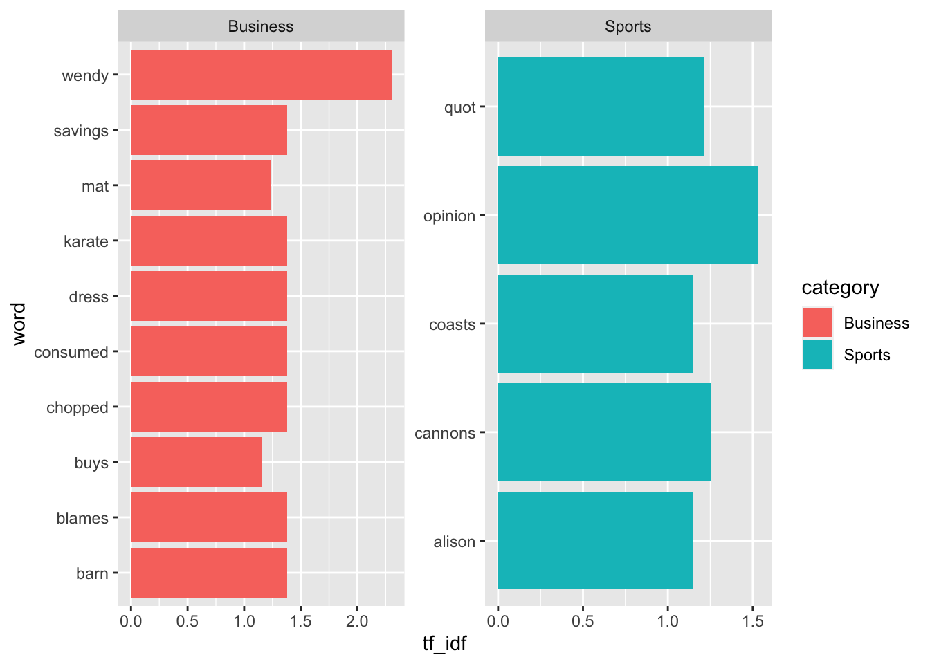
In the previous plot:
geom_colis the same asgeom_bar(stat="identity"): it plots a barplot without calculating the values (i.e., the values are already counted)scales = "free"allows each plot to have independent x and y axiscoord_flipflips the corrdinates so that we get the terms on the y-axis and the tf-idf scores on the x-axis
9.4 Removing sparse terms
In any real text dataset, we will have thousands of unique words. So creating a document term matrix with thousands of columns might not be the best choice as it will include a lot of noise. For instance, in this data, we have 5580 distinct words:
d2 %>% distinct(word) %>% nrow## [1] 5580Let’s assume that we want to focus only on words that appear at least in 15 documents:
focal_words = d2 %>% group_by(word) %>% count() %>% filter(n > 15)
focal_words %>% nrow
## [1] 141
Note that
d2is already grouped-by document, and as a result grouping by word (see above) counts how many times each word appears in each document
We can now keep only the focal_words by running an inner join, and then, by using pivot_wider, we can get the document-term matrix:
d2 %>% inner_join(focal_words, by="word") %>%
       pivot_wider(names_from = word, values_from = tf_idf, values_fill = 0) %>%
       arrange(desc(olympics))
## # A tibble: 3,856 × 144
## title category n quot san olympics million week pay bank hurricane
## <chr> <chr> <int> <dbl> <dbl> <dbl> <dbl> <dbl> <dbl> <dbl> <dbl>
## 1 At t… Sports 22 0 0 0.635 0 0 0 0 0
## 2 Gree… Sports 22 0 0 0.347 0 0 0 0 0
## 3 Oooh… Sports 22 0 0 0.347 0 0 0 0 0
## 4 Coac… Sports 22 0 0 0.318 0 0 0 0 0
## 5 Note… Sports 22 0 0 0.318 0 0 0 0 0
## 6 Time… Sports 22 0 0 0.318 0 0 0 0 0
## 7 Aust… Sports 22 0 0 0.293 0 0 0 0 0
## 8 Judg… Sports 22 0 0 0.293 0 0 0 0 0
## 9 Nest… Sports 22 0 0 0.293 0 0 0 0 0
## 10 El G… Sports 22 0 0 0.254 0 0 0 0 0
## # … with 3,846 more rows, and 133 more variables: growth <dbl>, months <dbl>,
## # plans <dbl>, billion <dbl>, florida <dbl>, oil <dbl>, biggest <dbl>,
## # start <dbl>, night <dbl>, jobs <dbl>, sales <dbl>, games <dbl>,
## # federal <dbl>, financial <dbl>, team <dbl>, history <dbl>, london <dbl>,
## # sunday <dbl>, economic <dbl>, earnings <dbl>, report <dbl>, quarter <dbl>,
## # athens <dbl>, season <dbl>, investment <dbl>, cut <dbl>, medal <dbl>,
## # profit <dbl>, rose <dbl>, percent <dbl>, gt <dbl>, lt <dbl>, …9.4.1 Sentiment analysis
Similar to what we did in the initial example with the three documents, we can perform an inner join between our tibble and the nrc_lexicon and then aggregate to get the overall sentiment of each document in our dataset:
d1 %>%  filter(str_detect(word,"^[a-z]+$")) %>%
        inner_join(nrc_lexicon, by="word") %>%
        count(title,sentiment) %>%
        pivot_wider(names_from = sentiment, values_from = n, values_fill = 0)
## # A tibble: 960 × 11
## title negative positive sadness trust anticipation joy surprise disgust
## <chr> <int> <int> <int> <int> <int> <int> <int> <int>
## 1 "'Canes … 1 2 1 1 0 0 0 0
## 2 "'Dream … 1 5 1 2 5 3 2 0
## 3 "'I'm 10… 0 3 0 2 1 1 0 0
## 4 "'Style'… 0 3 0 2 1 2 0 0
## 5 "(17) Ut… 0 1 0 4 1 1 0 0
## 6 "\\$616m… 1 0 0 0 1 0 0 1
## 7 "#39;Can… 0 1 0 0 1 0 0 0
## 8 "#39;Pro… 3 2 1 1 1 1 0 2
## 9 "#39;Spa… 1 1 0 0 1 0 0 0
## 10 "100 win… 0 3 0 1 0 0 0 0
## # … with 950 more rows, and 2 more variables: fear <int>, anger <int>For comments, suggestions, errors, and typos, please email me at: kokkodis@bc.edu