A Midterm practice exam
library(rtweet)
library(tidyverse)
library(ggplot2)
library(ggthemes)
library(rvest)
library(lubridate)
A.1 Essay question
Q1: If you were given a large (billions of records) dataset, what would you do to understand the quality and limitations of the data?
A: This is a question that basically is covered in the slides of week 2. Some of the things we can do to profile (big) datasets:
- Understand what each column stores.
- Figure out the correct data types.
- Identify if there are missing observations by running aggregate functions (such as
summary). - Use
head()andtail()to view the first and last 6 rows of the dataset. - Get descriptive statistics of each column (min, max, mean, std, median, frequencies of categorical variables, etc.)
- Group by different groups of interest and estimate descriptive statistics.
- Select the variables that we care about, and the observations we care about (filter, subsample).
- Identify what questions the data can potentially answer.
In the exam, any combination that would include 4 or more of these points would have gotten full points.
A.2 Twitter API: rtweet
Q2: Use the rtweet function get_timeline to get the most recent 3000 tweets of the main ESPN twitter account (username: espn). Then, use the function as_date from the package lubridate to customize column created_at to date. Finally, store into a new tibble named e1 the ESPN tweets posted in September. How many tweets did ESPN post in September?
A: First let’s create our token (keys excluded from knitted file with the option {r, include=FALSE}):
myToken = create_token(app = app_name,
             consumer_key = key,
             consumer_secret = secret,
             access_token = access,
             access_secret = access_secret)
One way to find the number of tweets of e1 is to call the function nrow():
e = get_timeline("espn", n = 3000, token =myToken)
e$approxDate = as_date(e$created_at)
e1 = e %>% filter(approxDate >= "2021-09-01" & approxDate <= "2021-09-30")
nrow(e1)
## [1] 516write_csv(e1 %>% select(source,retweet_name,favorite_count,retweet_count),"../data/tweetsPracticeExam.csv")Q3: How many columns does the tibble e1 have?
A: (alternatively you can just run e1 and look at the number of columns.)
ncol(e1) ## [1] 91Q4: Now load a subset of the ESPN tweets and columns from here: tweetsPracticeExam.csv. Name this tibble p. Which one is the most frequently used source that ESPN uses to tweet from?
A:
p = read_csv("../data/tweetsPracticeExam.csv")
p %>%  group_by(source) %>% count() %>% arrange(desc(n))
## # A tibble: 8 × 2
## # Groups: source [8]
## source n
## <chr> <int>
## 1 Sprinklr 492
## 2 Twitter for iPhone 146
## 3 Twitter Web App 92
## 4 TweetDeck 88
## 5 Twitter Media Studio 60
## 6 WSC Sports 41
## 7 Twitter for Advertisers (legacy) 12
## 8 Twitter Media Studio - LiveCut 12Q5: How many tweets from the p tibble are retweets (i.e., they have a name in column retweet_name?)
A:
p %>% filter(!is.na(retweet_name)) %>% nrow## [1] 297Q6: In the p tibble, match the times that each of the following account is being retweeted by ESPN:
A: Below I am using the operatore %in% to keep only rows where the retweet_name is one of the focal ones that the question asks. You did not have to do this to answer this question. You can answer the question without using the last filter.
p %>% filter(!is.na(retweet_name)) %>% group_by(retweet_name) %>% count() %>%
  arrange(n) %>%
  filter(retweet_name %in% c('DJ KHALED','Malika Andrews',
                             'ESPN College Football',
                             'NFL on ESPN',
                             'Adam Schefter',
                             'ESPN FC',
                             'ESPN Fantasy Sports'))
## # A tibble: 7 × 2
## # Groups: retweet_name [7]
## retweet_name n
## <chr> <int>
## 1 DJ KHALED 1
## 2 ESPN Fantasy Sports 2
## 3 Malika Andrews 2
## 4 ESPN College Football 5
## 5 Adam Schefter 15
## 6 ESPN FC 19
## 7 NFL on ESPN 24Q7: From the p tibble keep only tweets that are posted through the ‘Twitter Web App’ and the ‘Twitter for iPhone’ sources. Furthermore, remove any tweets that have fewer than 1 favorite_count and fewer than 1 retweet_count. Use ggplot2 to create a scatterplot where on the x-axis you have the log of favorite_count and on the y-axis the retweet_count. Add linear trend lines (method="lm") that show the trends of different sources. Use a theme of your choice. Which one of the two sources has a greater slope?
A:
myPallette = "Dark2"
ggplot(p %>% filter((source == 'Twitter Web App' | source == 'Twitter for iPhone') & (favorite_count > 1 & retweet_count > 1)) ,
                                    aes(x = log(favorite_count), y = retweet_count, color = source, shape=source, fill = source ))+
  geom_point()+theme_economist()+
  scale_fill_brewer(palette =myPallette)+geom_smooth(method="lm")+
  scale_color_brewer(palette =myPallette)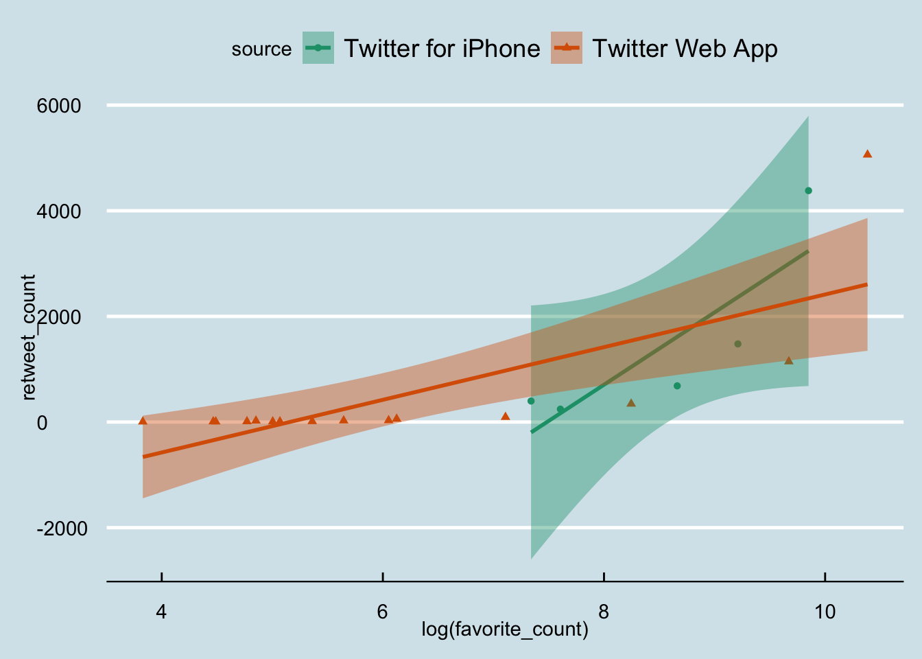
Q8: From the p tibble, store to a csv file only columns retweet_name, and retweet_count, and only those rows that represent retweets (retweet_name is not missing).
A:
write_csv(p %>% filter(!is.na(retweet_name)) %>% select(retweet_name,retweet_count), "../data/espnTweets.csv")A.3 Scraping
Q10: Scrape the URL: https://en.wikipedia.org/wiki/Data_analysis
Use the HTML tag “p a” to extract all the links on this page. Then use the regular expression “[a-zA-Z ]+” to keep only links that are not references. Save the result to a single-column tibble. Name the column “Relevant link”. Remove any missing values.
How many links did you end up with?
Note how to access columns with names that include spaces.
A:
r = read_html("https://en.wikipedia.org/wiki/Data_analysis")
r1 = r %>% html_nodes("p a") %>%
  html_text()
r2 = r1 %>% str_extract("[a-zA-Z ]+") %>% as_tibble_col("Relevant link") %>%
  filter(!is.na(`Relevant link`))
nrow(r2 )
## [1] 84Q11: Now use the regular expression “[0-9]+” to keep only numbers. Save the result to a single-column tibble. Name the column “Relevant number”.
Use the function parse_number(`Relevant number`) to update the type of column Relevant number to double.
The function
parse_numberwill remove any trailing characters, dollar signs, and commas and transform the input to numeric values (or NAs if non-numeric values are found).)
What is the mean of the column Relevant number?
r1 %>% str_extract("[0-9]+") %>% as_tibble_col("Relevant number") %>%
  mutate(`Relevant number` = parse_number(`Relevant number`)) %>%
  summarize(mean(`Relevant number`,na.rm=T))
## # A tibble: 1 × 1
## `mean(\`Relevant number\`, na.rm = T)`
## <dbl>
## 1 68.8Q12: Create a new custom function that:
- Takes as input a wiki concept.
- Visits its wikipedia page.
- Extracts all the links.
- Removes any missing values.
- Returns a tibble with two columns: the first column stores the link, and the second column stores the scraped wiki concept.
By using a function from the map() family, call your new custom function with the following wiki concepts as input:** c('Data_mining','Data_analysis','Data_science') Store the result into a single tibble.How many rows does this final tibble have?
A:
getWikis = function(wikiConcept){
  r = read_html(paste("https://en.wikipedia.org/wiki/",wikiConcept,sep=""))
  r1 = r %>% html_nodes("p a") %>% html_text()
  r2 = r1 %>% str_extract("[a-zA-Z ]+") %>% as_tibble_col("link") %>% filter(!is.na(link)) %>% mutate(concept = wikiConcept)
  return(r2)
}

d = c('Data_mining','Data_analysis','Data_science') %>% map_dfr(getWikis)
nrow(d)
## [1] 248For comments, suggestions, errors, and typos, please email me at: kokkodis@bc.edu