11 Predictive modeling II: Classification
In this chapter we will discuss how we can predict binary (categorical) dependent variables by performing basic classification analysis in R.
library(tidymodels)
library(tidyverse)
set.seed(7)
11.1 Data profiling
We will use a credit cards dataset. Our goal is to estimate the probability that a customer will pay their credit card debt given the customer’s observed characteristics.
d = read_csv("../data/creditCards.csv")
d
## # A tibble: 30,000 × 5
## TARGET GENDER MARRIAGE CREDIT_LIMIT AGE
## <chr> <dbl> <dbl> <dbl> <dbl>
## 1 NOT_PAID 2 1 20000 24
## 2 NOT_PAID 2 2 120000 26
## 3 PAID 2 2 90000 34
## 4 PAID 2 1 50000 37
## 5 PAID 1 1 50000 57
## 6 PAID 1 2 50000 37
## 7 PAID 1 2 500000 29
## 8 PAID 2 2 100000 23
## 9 PAID 2 1 140000 28
## 10 PAID 1 2 20000 35
## # … with 29,990 more rows11.1.1 Data types
The first thing to do is to verify that each column has the correct data type. Columns Gender and Marriage are listed as numeric whereas they should be categorical. Similarly, our dependent variable TARGET is listed as a character column. We will need to transform these columns into categorical (factors), in order for our models to work correctly.
d = d  %>%  mutate(across(c(TARGET,GENDER,MARRIAGE), factor))
d
## # A tibble: 30,000 × 5
## TARGET GENDER MARRIAGE CREDIT_LIMIT AGE
## <fct> <fct> <fct> <dbl> <dbl>
## 1 NOT_PAID 2 1 20000 24
## 2 NOT_PAID 2 2 120000 26
## 3 PAID 2 2 90000 34
## 4 PAID 2 1 50000 37
## 5 PAID 1 1 50000 57
## 6 PAID 1 2 50000 37
## 7 PAID 1 2 500000 29
## 8 PAID 2 2 100000 23
## 9 PAID 2 1 140000 28
## 10 PAID 1 2 20000 35
## # … with 29,990 more rowsCheck out Section 7.3.1 to recall how to use the function
across.
11.2 Feature engineering
This process will be similar to the one we introduced in the previous chapter, in Section 10.3.
11.2.1 Data spliting
Next, we will split our data into training and test sets:
ds = initial_split(d, prop=5/6)
trs = training(ds)
ts = testing(ds)
11.2.2 Recipes
Now we can use the training set to do some feature engineering. Recall that models do not understand categorical variables and that in order to use them we will need to transform them into binary columns which are called dummies. For our basic recipe in this example, we will use the function step_dummy that transforms all categorical columns into binary.
br = recipe(TARGET ~ GENDER + MARRIAGE + CREDIT_LIMIT + AGE, trs) %>%
     step_dummy(all_nominal(), -all_outcomes())
br %>% prep %>% juice %>% summary
## CREDIT_LIMIT AGE TARGET GENDER_X2
## Min. : 10000 Min. :21.00 NOT_PAID: 5568 Min. :0.000
## 1st Qu.: 50000 1st Qu.:28.00 PAID :19432 1st Qu.:0.000
## Median :140000 Median :34.00 Median :1.000
## Mean :167586 Mean :35.45 Mean :0.604
## 3rd Qu.:240000 3rd Qu.:41.00 3rd Qu.:1.000
## Max. :800000 Max. :75.00 Max. :1.000
## MARRIAGE_X1 MARRIAGE_X2 MARRIAGE_X3
## Min. :0.0000 Min. :0.0000 Min. :0.00000
## 1st Qu.:0.0000 1st Qu.:0.0000 1st Qu.:0.00000
## Median :0.0000 Median :1.0000 Median :0.00000
## Mean :0.4538 Mean :0.5337 Mean :0.01076
## 3rd Qu.:1.0000 3rd Qu.:1.0000 3rd Qu.:0.00000
## Max. :1.0000 Max. :1.0000 Max. :1.00000Furthermore, we can create an additional recipe which extends our basic recipe by log-transforming the credit limit:
er = br %>% step_log(CREDIT_LIMIT)
er %>%  prep %>% juice %>% head
## # A tibble: 6 × 7
## CREDIT_LIMIT AGE TARGET GENDER_X2 MARRIAGE_X1 MARRIAGE_X2 MARRIAGE_X3
## <dbl> <dbl> <fct> <dbl> <dbl> <dbl> <dbl>
## 1 12.1 30 PAID 1 0 1 0
## 2 11.5 32 NOT_PAID 1 1 0 0
## 3 11.7 40 PAID 1 1 0 0
## 4 10.8 35 PAID 1 1 0 0
## 5 12.8 35 PAID 1 1 0 0
## 6 9.90 30 NOT_PAID 1 1 0 011.3 Classification models
Defining classification models is very similar to defining regression models (Section 10.4.2). Specifically, we will need to use the model’s special keyword, the function set_engine which identify which package to use, and the function set_mode which identifies whether this is a regression or a classification problem. Here we define five classification models:
dt_class = decision_tree() %>% set_engine("rpart") %>% set_mode("classification")
xg_class = boost_tree() %>% set_engine("xgboost") %>% set_mode("classification")
lg_class =  logistic_reg() %>% set_engine("glm") %>% set_mode("classification")
mlp_class = mlp() %>% set_engine("keras") %>% set_mode("classification")
rf_class = rand_forest() %>% set_engine("ranger") %>% set_mode("classification")
Next, we define a basic workflow:
bw = workflow() %>% add_model(lg_class) %>% add_recipe(br)
bw
## ══ Workflow ═══════════════════════════════════════════════════════════════════════════════════════════════════════════════════════════════════════════════════════════════════════
## Preprocessor: Recipe
## Model: logistic_reg()
##
## ── Preprocessor ───────────────────────────────────────────────────────────────────────────────────────────────────────────────────────────────────────────────────────────────────
## 1 Recipe Step
##
## • step_dummy()
##
## ── Model ──────────────────────────────────────────────────────────────────────────────────────────────────────────────────────────────────────────────────────────────────────────
## Logistic Regression Model Specification (classification)
##
## Computational engine: glmFinally, we can call function fit on the training set to train these models, and the function predict to get our predictions for the test set:
logitFit = bw %>% fit(trs)
p = predict(logitFit, ts) %>%  bind_cols(ts %>% select(TARGET))
p
## # A tibble: 5,000 × 2
## .pred_class TARGET
## <fct> <fct>
## 1 PAID PAID
## 2 PAID PAID
## 3 PAID NOT_PAID
## 4 PAID PAID
## 5 PAID NOT_PAID
## 6 PAID PAID
## 7 PAID PAID
## 8 PAID PAID
## 9 PAID PAID
## 10 PAID NOT_PAID
## # … with 4,990 more rows11.4 Evaluation
Now that we have built our classification models, how do we know which ones work and which ones do not work?
In classification, we care about whether or not we can correctly predict class membership. For instance, we want to know whether or not a customer is more likely to pay or not pay their credit card bills. Hence, for these types of models (i.e., classification models), we use the following evaluation metrics:
Accuracy and confusion matrix: The accuracy of a classifier quantifies the ratio of corrected classified instances. The accuracy is a direct result of a model’s confusion matrix, which captures the number of true positives, true negatives, false positives, and false negatives.
AUC, sensitivity, specificity: Pretty often, the accuracy of a classifier can be misleading. In those cases, a metric such as the AUC (Area Under the Curve, or Area Under the ROC curve, or ROC)—which captures the correctness of our predicted membership probabilities and subsequent rankings are—is more appropriate. The AUC metric is a direct result of sensitivity and specificity, two metrics that capture the performance of an algorithm within each available class.
11.4.1 Accuracy and confusion matrix
A True Positive (TP) is an instance that was predicted positive and it is actually positive. A True Negative (TN) is an instance that was predictive negative and it is actually negative. False Positives (FP) and False Negatives (FN) capture errors that our classifiers make. A FP is an instance that was predicted positive but it is actually negative. Finally, a FN is an instance that was predicted to be negative but it is actually positive.
If we put the number of TP, TN, FP and FN in a table, we can get the confusion matrix by calling the function conf_mat from the package yardstick. The result looks like this:
p %>% conf_mat(TARGET,.pred_class)## Truth
## Prediction NOT_PAID PAID
## NOT_PAID 0 0
## PAID 1068 3932The confusion matrix has three columns: the first column lists the predicted classes. The other two columns list the negative and the positive observed instances in the test set. The elements in the confusion matrix identify the number that predictions and observations agree and disagree, and hence identify the TPs, TNs, FPs, and FNs.
In this example, negative instances are the
NOT_PAIDinstances, while positive instances are thePAIDones.
From the confusion matrix, we can get the accuracy by summing the diagonal and dividing by the total number of instances in our test set. Or simpler, by calling the function accuracy:
p %>% accuracy(TARGET,.pred_class)## # A tibble: 1 × 3
## .metric .estimator .estimate
## <chr> <chr> <dbl>
## 1 accuracy binary 0.78611.4.2 AUC
Some times, the accuracy of a classifier can be misleading. In our example, the accuracy is close to ~80%. Yet, our classifier never predicts customers who will not pay their debts (never predicts NOT_PAID). As a result, our model is majority class classifier.
Thankfully, we can use a different evaluation metric that is not affected by how skewed towards one class our input distribution is. This metric is caller Area Under the ROC Curve (AUC). The AUC describes the ability of a classifier to separate instances. Intuitively, the AUC score captures the probability that a randomly chosen positive instance from our dataset will rank higher than a randomly chosen negative one. Specifically, the AUC score is the area under a curve that captures the relationship between the true positive rate (sensitivity) and the false positive rate (1-specificity) of a classifier. To understand this, we first need to talk about thresholds and probabilities.
Most classifiers predict class membership probabilities. This means that they predict the likelihood that each point will be positive or negative. For instance in our example, a probabilistic classifier will predict the likelihood of a customer to pay their credit card bill. Hence, in order to map these probabilities to classes, we need to set up a threshold, such that a probability estimate above that threshold signals a fraudulent transaction, and a probability estimate below that threshold signals a legitimate transaction.
To get the probability estimates of our predictions, we need to call the function predict with the option prob:
p = predict(logitFit, ts, "prob") %>% bind_cols(ts %>% select(TARGET))
p %>% head
## # A tibble: 6 × 3
## .pred_NOT_PAID .pred_PAID TARGET
## <dbl> <dbl> <fct>
## 1 0.171 0.829 PAID
## 2 0.152 0.848 PAID
## 3 0.272 0.728 NOT_PAID
## 4 0.271 0.729 PAID
## 5 0.252 0.748 NOT_PAID
## 6 0.307 0.693 PAIDNow, we can call the function roc_curve which will estimate the AUC score of our model, by adjusting the probability threshold from 0 to 1 and plotting the sensitivity and the 1-specificity curve. Our curve looks like this:
p %>% roc_curve(truth = TARGET, .pred_PAID, event_level = "second") %>% autoplot()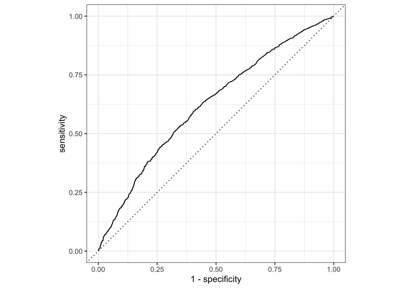
The area under this curve can be estimated by the function roc_auc as follows:
p %>% roc_auc(truth = TARGET, .pred_PAID, event_level = "second")## # A tibble: 1 × 3
## .metric .estimator .estimate
## <chr> <chr> <dbl>
## 1 roc_auc binary 0.622levels(p$TARGET)## [1] "NOT_PAID" "PAID"
event_level = "second". This basically identifies whether we want to rank the predicted instances according to their likelihood of “PAID” or “NOT_PAID”. The event_level can be set to either first or second. In our case, we want to rank instances according to their likelihood of being PAID. If we check the order of level PAID in our dependent variable TARGET (see previous chunk) we will notice that it comes second. Hence, we set event_level = "second".
11.4.3 Comparison of multiple models
Next, we define a function evalClass that streamlines the process of estimating the AUC score of different algorithms. The function takes as input a workflow, and returns the AUC score estimated on the test set of the model included in the workflow:
evalClass = function(aWorkFlow){
  tmpFit = aWorkFlow %>% fit(trs)
  p = predict(tmpFit, ts, "prob") %>%  bind_cols(ts %>% select(TARGET))
  p %>% roc_auc(truth = TARGET, .pred_PAID, event_level = "second")
}
We can call this function multiple times and create a final tibble that includes the results.
r1 = bw %>% evalClass %>% mutate(model = "logit",recipe="b")
r2 = bw %>% update_recipe(er) %>%  evalClass  %>% mutate(model = "logit",recipe="e")
r3 = bw %>% update_model(rf_class) %>% evalClass  %>%mutate(model = "rf",recipe="b")
r4 = bw %>% update_model(rf_class) %>% update_recipe(er) %>%evalClass  %>% mutate(model = "rf",recipe="e")
r = bind_rows(r1,r2,r3,r4)
r
## # A tibble: 4 × 5
## .metric .estimator .estimate model recipe
## <chr> <chr> <dbl> <chr> <chr>
## 1 roc_auc binary 0.622 logit b
## 2 roc_auc binary 0.628 logit e
## 3 roc_auc binary 0.626 rf b
## 4 roc_auc binary 0.626 rf eFinally, we can plot the results in a bar plot:
r %>% ggplot(aes(x=model, y = .estimate, fill = model) )+geom_col() + facet_wrap(~recipe)
11.5 Threshold analysis
The previous discussion about thresholds and probabilities raises another question:
How do we choose a threshold in practice?
The answer is it depends: it depends on what we care for. Do we care about minimizing the number of FPs? Or do we care about minimize the number of FNs? Or do we equally care about minimizing both FPs and FNs at the same time? Sensitivity and Specificity are good measures to optimize depending on what our objective is:
Sensitivity is defined as the number of TPs over the number of positives, and it captures the probability of correctly classifying an instance given that it is positive. As a result sensitivity is a measure we want to maximize when we care about minimizing the number of FNs!!
On the other hand, specificity is defined as the number of TNs over the total number of negatives, and it captures the probability of correctly classifying an instance given that it is negative. As a result, specificity is a measure we want to maximize when we care about minimizing the number of FPs.
To perform this analysis in R, we will use the package probably:
install.packages("probably")library(probably)Let’s get the probability estimates of our model:
p = predict(logitFit, ts, "prob") %>%  bind_cols(ts %>% select(TARGET))
p %>%  head
## # A tibble: 6 × 3
## .pred_NOT_PAID .pred_PAID TARGET
## <dbl> <dbl> <fct>
## 1 0.171 0.829 PAID
## 2 0.152 0.848 PAID
## 3 0.272 0.728 NOT_PAID
## 4 0.271 0.729 PAID
## 5 0.252 0.748 NOT_PAID
## 6 0.307 0.693 PAIDThe function threshold_perf will use these probability estimates to compute the sensitivity, specificity, and j index for different thresholds:
thresholdData = p %>% threshold_perf(TARGET, .pred_PAID, thresholds = seq(0.2,0.8, by=0.0025))
thresholdData %>% head
## # A tibble: 6 × 4
## .threshold .metric .estimator .estimate
## <dbl> <chr> <chr> <dbl>
## 1 0.2 sens binary 1
## 2 0.202 sens binary 1
## 3 0.205 sens binary 1
## 4 0.208 sens binary 1
## 5 0.21 sens binary 1
## 6 0.213 sens binary 1
When we care about both the sensitivity and the specificity of a model, we can use the J-index. The J-index can provide a sort of best-threshold point where increasing the threshold results in no more of an increase in the specificity than a decrease in the sensitivity, and as a result the J-index is maximized. We can plot these metrics as follows:
thresholdData %>% ggplot(aes(x=.threshold, y =.estimate, color =.metric))+geom_line()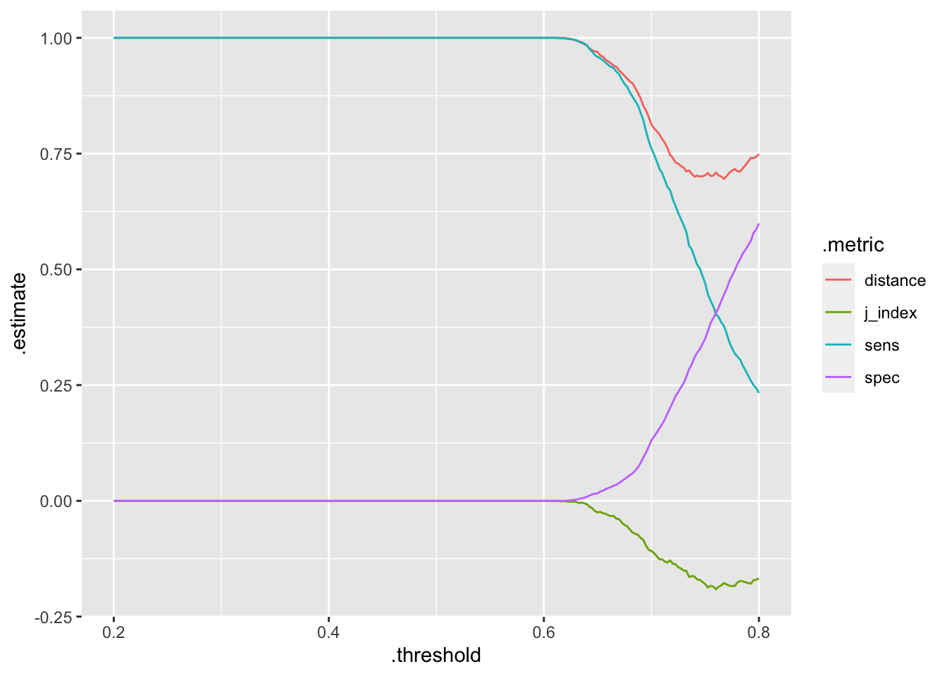
Then, we can get the thresholds that maximize the J index:
thresholdData %>% filter(.metric == "j_index") %>% filter(.estimate == max(.estimate)) %>% head## # A tibble: 6 × 4
## .threshold .metric .estimator .estimate
## <dbl> <chr> <chr> <dbl>
## 1 0.2 j_index binary 0
## 2 0.202 j_index binary 0
## 3 0.205 j_index binary 0
## 4 0.208 j_index binary 0
## 5 0.21 j_index binary 0
## 6 0.213 j_index binary 0For comments, suggestions, errors, and typos, please email me at: kokkodis@bc.edu