14 Predicting high spenders in an e-commerce platform
In this final chapter we will use many of the concepts we have covered in this book to build a predictive algorithm that estimates the likelihood of a user to become a high spender. To do so, we will use data from the e-commerce platform JD.com, which is China’s largest retailer with a net revenue of 67.2 billion USD in 2018 and over 320 million annual active customers. In particular we will use two datasets: the users dataset, which stores information about the platforms users, and the orders dataset, which stores information about orders placed by each user.
Our goal is simple: can we predict if a user will be a high spender based on the user’s observed characteristics? If we can, the JD.com can focus on targeting these users, or even attract more users that are likely to become high spenders.
library(tidymodels)
library(tidyverse)
library(lubridate)
library(ggthemes)
library(probably)
In this chapter
14.1 Data profiling
Let’s first profile these datasets:
orders = read_csv("../data/orders.csv")
users = read_csv("../data/users.csv")
users %>% head## # A tibble: 6 × 10
## user_ID user_level first_order_month plus gender age marital_status
## <chr> <dbl> <chr> <dbl> <chr> <chr> <chr>
## 1 000089d6a6 1 2017-08 0 F 26-35 S
## 2 0000babd1f 1 2018-03 0 U U U
## 3 0000bc018b 3 2016-06 0 F >=56 M
## 4 0000d0e5ab 3 2014-06 0 M 26-35 M
## 5 0000dce472 3 2012-08 1 U U U
## 6 0000f81d1b 1 2018-02 0 F 26-35 M
## # … with 3 more variables: education <dbl>, city_level <dbl>,
## # purchase_power <dbl>The column first_order_month is of type character; however, it sores date-relevant information. We will use the as_date function to transform it into a date type:
as_date(paste("2017-08","-15",sep=""), format = "%Y-%m-%d")## [1] "2017-08-15"users$first_order_month = as_date(paste(users$first_order_month,"-15", sep=""),
format = "%Y-%m-%d")Multiple variables need to be transformed into categorical variables. In addition, some variables are irrelevant to our problem, as they are market-specific. We can remove those with a dash inside a select:
users = users %>% mutate(across(c(gender, age,marital_status,education), factor)) %>%
      select(-c(city_level,purchase_power,user_level,plus))
users %>%  head
## # A tibble: 6 × 6
## user_ID first_order_month gender age marital_status education
## <chr> <date> <fct> <fct> <fct> <fct>
## 1 000089d6a6 2017-08-15 F 26-35 S 3
## 2 0000babd1f 2018-03-15 U U U -1
## 3 0000bc018b 2016-06-15 F >=56 M 3
## 4 0000d0e5ab 2014-06-15 M 26-35 M 3
## 5 0000dce472 2012-08-15 U U U -1
## 6 0000f81d1b 2018-02-15 F 26-35 M 2From the orders dataset, we will estimate the total money spent of each user on the platform. This will become our dependent variable:
orders = orders %>% group_by(user_ID) %>% summarize(totalSpent = sum(final_unit_price))Now we can join the two datasets and create our final tibble, which will store information about each user along with each user’s total amount of money spent.
f = users %>% inner_join(orders, by="user_ID")
f %>%  head
## # A tibble: 6 × 7
## user_ID first_order_month gender age marital_status education totalSpent
## <chr> <date> <fct> <fct> <fct> <fct> <dbl>
## 1 000089d6a6 2017-08-15 F 26-35 S 3 215
## 2 0000babd1f 2018-03-15 U U U -1 39
## 3 0000bc018b 2016-06-15 F >=56 M 3 79
## 4 0000d0e5ab 2014-06-15 M 26-35 M 3 228
## 5 0000dce472 2012-08-15 U U U -1 112.
## 6 0000f81d1b 2018-02-15 F 26-35 M 2 150Some instances of our final dataset have errors; Specifically, there are customers who have spent a negative amount of money. We will drop these observations:
f1 = f %>% filter(totalSpent > 1)
f1 %>% summary
## user_ID first_order_month gender age
## Length:403506 Min. :2003-12-15 F:263528 <=15 : 20
## Class :character 1st Qu.:2014-05-15 M: 90010 >=56 : 12955
## Mode :character Median :2016-03-15 U: 49968 16-25: 91748
## Mean :2015-09-07 26-35:161056
## 3rd Qu.:2017-07-15 36-45: 71788
## Max. :2018-03-15 46-55: 16689
## U : 49250
## marital_status education totalSpent
## M:161878 -1: 96452 Min. : 1.05
## S:159074 1 : 7102 1st Qu.: 49.00
## U: 82554 2 : 64309 Median : 69.00
## 3 :193175 Mean : 97.60
## 4 : 42468 3rd Qu.: 121.00
## Max. :81977.92
## Let’s visualize our dependent variable:
f1 %>% ggplot(aes(x=totalSpent))+geom_density()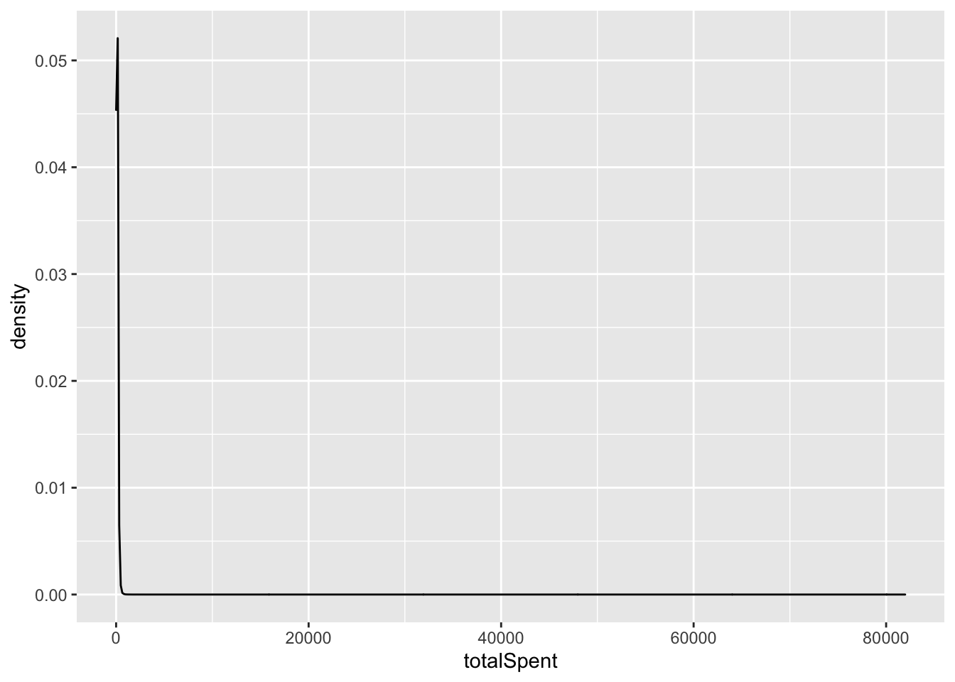
This plot shows that the majority of customers spent very little. However, there are a few customers who spend a tremendous amount of money. As a result, the distribution of the total amount spent has a very long tail (power law). Let’s log-transform it to see if it looks better:
f1$totalSpent = log(f1$totalSpent)
f1 %>% ggplot(aes(x=totalSpent))+geom_density()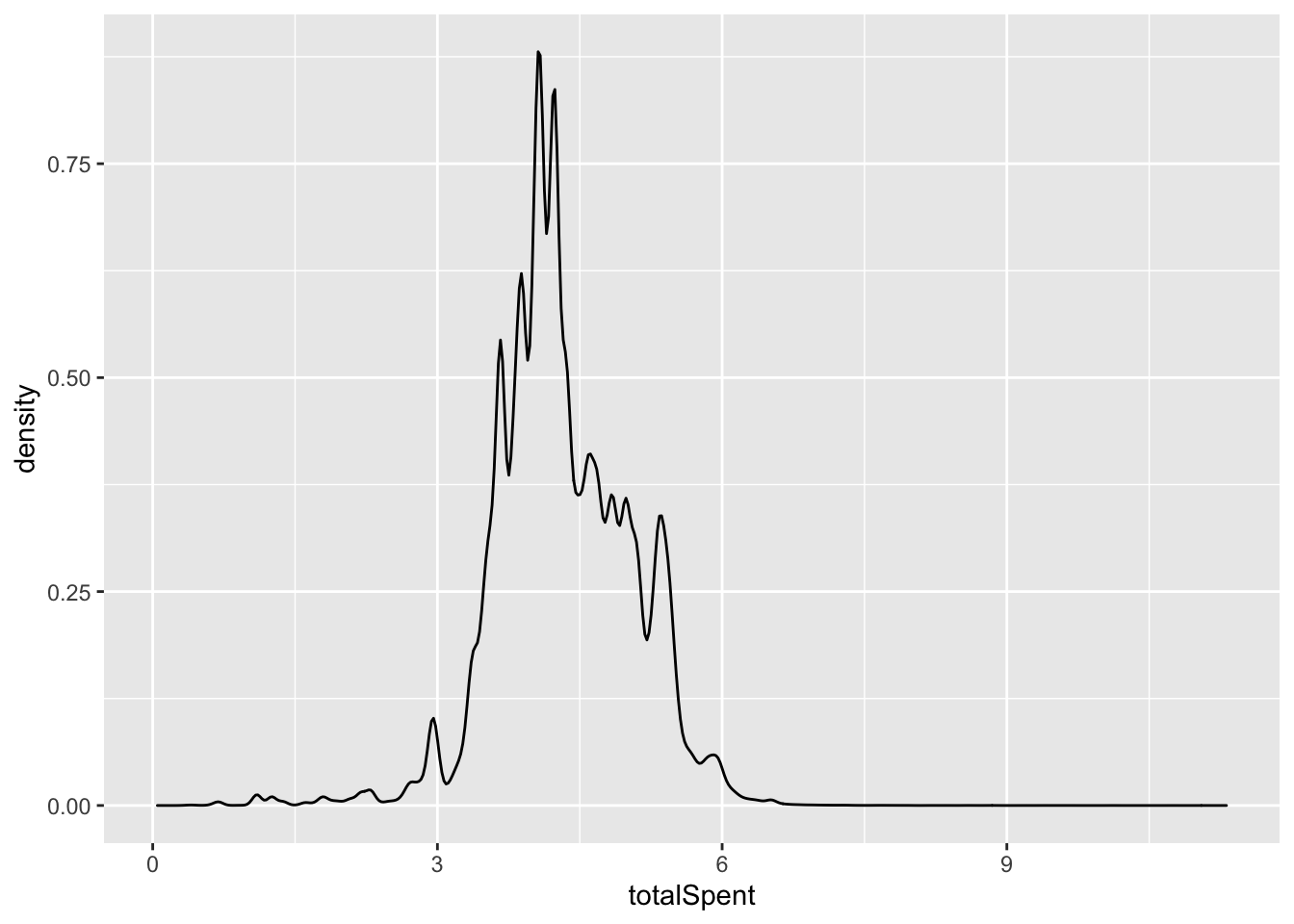
Furthermore, some of the variables have missing values, in the form of “-1” or “U”. We will need to replace these values with NA so that we can impute them in the next step:
f1 = f1 %>% mutate(education = na_if(education,"-1"), marital_status = na_if(marital_status, "U")) %>%
        mutate(education = factor(education, levels = c("1","2","3", "4")), marital_status = factor(marital_status, levels= c("S","M")) )
f1 %>% head
## # A tibble: 6 × 7
## user_ID first_order_month gender age marital_status education totalSpent
## <chr> <date> <fct> <fct> <fct> <fct> <dbl>
## 1 000089d6a6 2017-08-15 F 26-35 S 3 5.37
## 2 0000babd1f 2018-03-15 U U <NA> <NA> 3.66
## 3 0000bc018b 2016-06-15 F >=56 M 3 4.37
## 4 0000d0e5ab 2014-06-15 M 26-35 M 3 5.43
## 5 0000dce472 2012-08-15 U U <NA> <NA> 4.71
## 6 0000f81d1b 2018-02-15 F 26-35 M 2 5.01Now because this dataset is huge, we will use a simple regular expression to subsample it and build my models:
tt = f1 %>% filter(str_detect(user_ID, "^[0-9]+$|(^[a])"))
tt %>% nrow
## [1] 2896914.2 Regression analysis
First, let’s assume that our goal is to predict the total money spent. Our dependent variable will be the column totalSpent.
14.2.1 Feature engineering
Now we are ready to split our data and define our recipes:
splits = initial_split(tt, prop = 4/5)
trs = training(splits)
ts = testing(splits)
Our recipe here uses all the available information and imputes all missing values with their columns’ median values.
br = recipe(totalSpent ~ gender + age +  marital_status + education,
            trs) %>%
  step_dummy(all_nominal()) %>%
  step_medianimpute(marital_status_M,education_X2, education_X3,
                    education_X4)
br %>% prep %>% juice %>% summary
## totalSpent gender_M gender_U age_X..56
## Min. :0.04879 Min. :0.0000 Min. :0.0000 Min. :0.00000
## 1st Qu.:3.89182 1st Qu.:0.0000 1st Qu.:0.0000 1st Qu.:0.00000
## Median :4.23411 Median :0.0000 Median :0.0000 Median :0.00000
## Mean :4.31948 Mean :0.2216 Mean :0.1272 Mean :0.03137
## 3rd Qu.:4.80402 3rd Qu.:0.0000 3rd Qu.:0.0000 3rd Qu.:0.00000
## Max. :9.15816 Max. :1.0000 Max. :1.0000 Max. :1.00000
## age_X16.25 age_X26.35 age_X36.45 age_X46.55
## Min. :0.0000 Min. :0.0000 Min. :0.0000 Min. :0.00000
## 1st Qu.:0.0000 1st Qu.:0.0000 1st Qu.:0.0000 1st Qu.:0.00000
## Median :0.0000 Median :0.0000 Median :0.0000 Median :0.00000
## Mean :0.2239 Mean :0.4035 Mean :0.1757 Mean :0.03974
## 3rd Qu.:0.0000 3rd Qu.:1.0000 3rd Qu.:0.0000 3rd Qu.:0.00000
## Max. :1.0000 Max. :1.0000 Max. :1.0000 Max. :1.00000
## age_U marital_status_M education_X2 education_X3
## Min. :0.0000 Min. :0.0000 Min. :0.0000 Min. :0.0000
## 1st Qu.:0.0000 1st Qu.:0.0000 1st Qu.:0.0000 1st Qu.:0.0000
## Median :0.0000 Median :1.0000 Median :0.0000 Median :1.0000
## Mean :0.1257 Mean :0.6113 Mean :0.1569 Mean :0.7136
## 3rd Qu.:0.0000 3rd Qu.:1.0000 3rd Qu.:0.0000 3rd Qu.:1.0000
## Max. :1.0000 Max. :1.0000 Max. :1.0000 Max. :1.0000
## education_X4
## Min. :0.0000
## 1st Qu.:0.0000
## Median :0.0000
## Mean :0.1108
## 3rd Qu.:0.0000
## Max. :1.000014.2.2 Model definition and training
Below we define three different regression models:
boost_reg = boost_tree()  %>%
  set_engine("xgboost")  %>%
  set_mode("regression")
dt_reg = decision_tree()  %>%
  set_engine("rpart")  %>%
  set_mode("regression")
mlp_reg = mlp()  %>%
  set_engine("keras")  %>%
  set_mode("regression")
bw = workflow() %>% add_model(boost_reg) %>% add_recipe(br)The function evalRegression is an adaptation of the regression function presented in Section 10.5.2.
evalRegression = function(curWorkflow){
  c = curWorkflow %>% fit(data=trs)
  p1 = predict(c, ts) %>%
  bind_cols(ts %>% select(totalSpent))
  t1 = p1 %>% mae(.pred, totalSpent)
  t2 = p1 %>% rmse(.pred, totalSpent)
  return(bind_rows(t1,t2))
}
14.2.3 Results
Let’s get the results:
l1 = bw %>% evalRegression %>% mutate(model = "xg")
l2 = bw %>% update_model(mlp_reg) %>%  evalRegression %>%
  mutate(model = "mlp")
l3= bw %>% update_model(dt_reg) %>%  evalRegression %>%
  mutate(model = "dt")
l = bind_rows(l1,l2,l3)
l
## # A tibble: 6 × 4
## .metric .estimator .estimate model
## <chr> <chr> <dbl> <chr>
## 1 mae standard 0.543 xg
## 2 rmse standard 0.704 xg
## 3 mae standard 0.544 mlp
## 4 rmse standard 0.703 mlp
## 5 mae standard 0.547 dt
## 6 rmse standard 0.706 dtAs we can see, all models seem to perform about the same:
l %>% ggplot(aes(x=model, y=.estimate, fill = model))+
  geom_col() + facet_wrap(~.metric)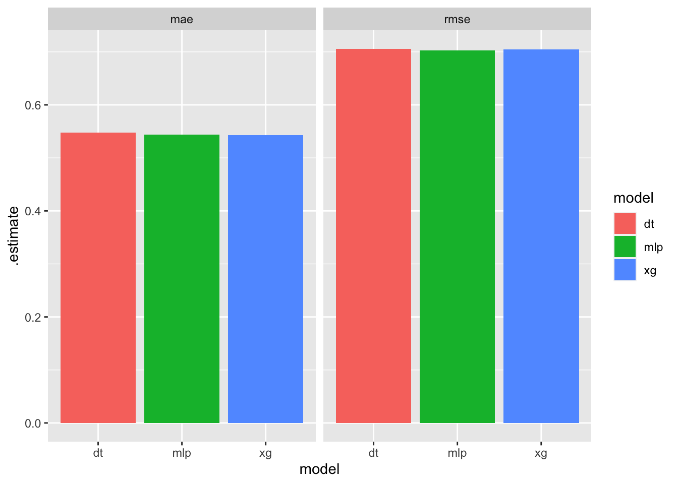
14.3 Classification
Now let’s transform this problem into a classification problem. To do so, we will need to binarize the variable totalSpent. Specifically, we can assume that customers who spend more than the median amount are high spenders, while those who spend less than the median are low spenders:
c = tt %>% mutate(highLow = ifelse(totalSpent > median(totalSpent),
                                   "high","low")) %>%
  select(-totalSpent) %>%
  mutate(highLow = factor(highLow, levels=c("high","low")))
c %>%  select(user_ID, highLow) %>%  head
## # A tibble: 6 × 2
## user_ID highLow
## <chr> <fct>
## 1 0009796280 high
## 2 0012371678 high
## 3 0014338531 low
## 4 0017950650 high
## 5 0022080047 low
## 6 0022307877 high14.3.1 Feature engineering
We will follow the same process as before:
splits = initial_split(c, prop = 4/5)
trs = training(splits)
ts = testing(splits)
br = recipe(highLow ~ gender + age + marital_status + education, trs) %>%
step_dummy(all_nominal(), -all_outcomes()) %>%
step_medianimpute(marital_status_M,education_X2, education_X3, education_X4)
br %>% prep %>% juice %>% summary## highLow gender_M gender_U age_X..56
## high:11163 Min. :0.0000 Min. :0.0000 Min. :0.0000
## low :12012 1st Qu.:0.0000 1st Qu.:0.0000 1st Qu.:0.0000
## Median :0.0000 Median :0.0000 Median :0.0000
## Mean :0.2216 Mean :0.1268 Mean :0.0318
## 3rd Qu.:0.0000 3rd Qu.:0.0000 3rd Qu.:0.0000
## Max. :1.0000 Max. :1.0000 Max. :1.0000
## age_X16.25 age_X26.35 age_X36.45 age_X46.55
## Min. :0.000 Min. :0.000 Min. :0.0000 Min. :0.00000
## 1st Qu.:0.000 1st Qu.:0.000 1st Qu.:0.0000 1st Qu.:0.00000
## Median :0.000 Median :0.000 Median :0.0000 Median :0.00000
## Mean :0.225 Mean :0.401 Mean :0.1778 Mean :0.03918
## 3rd Qu.:0.000 3rd Qu.:1.000 3rd Qu.:0.0000 3rd Qu.:0.00000
## Max. :1.000 Max. :1.000 Max. :1.0000 Max. :1.00000
## age_U marital_status_M education_X2 education_X3
## Min. :0.0000 Min. :0.0000 Min. :0.0000 Min. :0.0000
## 1st Qu.:0.0000 1st Qu.:0.0000 1st Qu.:0.0000 1st Qu.:0.0000
## Median :0.0000 Median :1.0000 Median :0.0000 Median :1.0000
## Mean :0.1252 Mean :0.6084 Mean :0.1579 Mean :0.7161
## 3rd Qu.:0.0000 3rd Qu.:1.0000 3rd Qu.:0.0000 3rd Qu.:1.0000
## Max. :1.0000 Max. :1.0000 Max. :1.0000 Max. :1.0000
## education_X4
## Min. :0.000
## 1st Qu.:0.000
## Median :0.000
## Mean :0.107
## 3rd Qu.:0.000
## Max. :1.00014.3.2 Model definition and training
We will use the exact same models as before, only now we will set_mode to classification:
boost_class = boost_tree()  %>%
  set_engine("xgboost")  %>%
  set_mode("classification")
dt_class = decision_tree()  %>%
  set_engine("rpart")  %>%
  set_mode("classification")
mlp_class = mlp()  %>%
  set_engine("keras")  %>%
  set_mode("classification")
bw = workflow() %>% add_model(boost_class) %>% add_recipe(br)#to identify the correct event level.
levels(c$highLow)## [1] "high" "low"evalClass = function(aWorkFlow){
tmpFit = aWorkFlow %>% fit(trs)
p = predict(tmpFit, ts, "prob") %>%
bind_cols(ts %>% select(highLow))
p %>% roc_auc(truth = highLow, .pred_high, event_level = "first")
}c1 = bw %>% evalClass %>% mutate(model = "xg")## [20:09:56] WARNING: amalgamation/../src/learner.cc:1095: Starting in XGBoost 1.3.0, the default evaluation metric used with the objective 'binary:logistic' was changed from 'error' to 'logloss'. Explicitly set eval_metric if you'd like to restore the old behavior.c2 = bw %>% update_model(mlp_class) %>% evalClass %>% mutate(model = "mlp")
c3 = bw %>% update_model(dt_class) %>% evalClass %>% mutate(model = "dt")bind_rows(c1,c2,c3)## # A tibble: 3 × 4
## .metric .estimator .estimate model
## <chr> <chr> <dbl> <chr>
## 1 roc_auc binary 0.562 xg
## 2 roc_auc binary 0.561 mlp
## 3 roc_auc binary 0.550 dt14.3.3 Threshold analysis
Now let’s see what threshold is best for our main model:
probs = bw %>% fit(trs) %>%  predict(ts, "prob") %>%
  bind_cols(ts %>% select(highLow))
## [20:10:05] WARNING: amalgamation/../src/learner.cc:1095: Starting in XGBoost 1.3.0, the default evaluation metric used with the objective 'binary:logistic' was changed from 'error' to 'logloss'. Explicitly set eval_metric if you'd like to restore the old behavior.td = threshold_perf(probs, highLow, .pred_high,
thresholds = seq(0.1,0.9, by=0.025))ggplot(td,aes(x=.threshold, y = .estimate, color = .metric))+geom_line()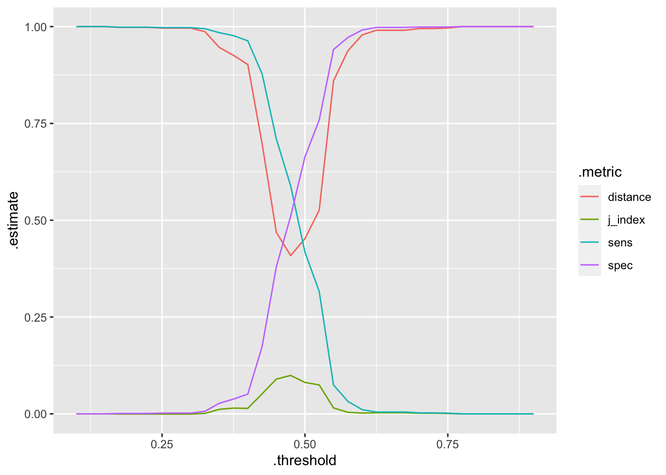
td %>% filter(.metric == "j_index") %>% filter(.estimate == max(.estimate))## # A tibble: 1 × 4
## .threshold .metric .estimator .estimate
## <dbl> <chr> <chr> <dbl>
## 1 0.475 j_index binary 0.0992Setting a threshold equal to 0.475 maximizes the J index!