10 Predictive modeling I: Regression
In this chapter we will discuss how we can predict continuous dependent variables by performing basic regression analysis in R. We will rely on a new package, tidymodels:
install.packages("tidymodels")library(tidymodels)
library(mlbench)
library(tidyverse)
We have previously installed pacakge
mlbenchin Section 1.7.
set.seed() to control the randomization process and get the same results every time we run the code from beginning to end.
set.seed(3)The goal of this exercise is to predict the glucose level given a set of features. Specifically, we want to learn the formula:
\(glucose \sim pressure + triceps + insulin + mass + pedigree + age + pregnant\)
10.1 Data profiling
To do so we will use a built-in diabetes dataset. This dataset comes from the mlbench package. We can load this with the data() function as follows:
data("PimaIndiansDiabetes")
d = as_tibble(PimaIndiansDiabetes)
Then we will drop the column diabetes as it is defined by the glucose level (and hence we would be cheating if we were to include it in our regression equation above):
d = d %>% select(-diabetes)
d
## # A tibble: 768 × 8
## pregnant glucose pressure triceps insulin mass pedigree age
## <dbl> <dbl> <dbl> <dbl> <dbl> <dbl> <dbl> <dbl>
## 1 6 148 72 35 0 33.6 0.627 50
## 2 1 85 66 29 0 26.6 0.351 31
## 3 8 183 64 0 0 23.3 0.672 32
## 4 1 89 66 23 94 28.1 0.167 21
## 5 0 137 40 35 168 43.1 2.29 33
## 6 5 116 74 0 0 25.6 0.201 30
## 7 3 78 50 32 88 31 0.248 26
## 8 10 115 0 0 0 35.3 0.134 29
## 9 2 197 70 45 543 30.5 0.158 53
## 10 8 125 96 0 0 0 0.232 54
## # … with 758 more rowsLet’s see how this data looks:
d %>% summary## pregnant glucose pressure triceps
## Min. : 0.000 Min. : 0.0 Min. : 0.00 Min. : 0.00
## 1st Qu.: 1.000 1st Qu.: 99.0 1st Qu.: 62.00 1st Qu.: 0.00
## Median : 3.000 Median :117.0 Median : 72.00 Median :23.00
## Mean : 3.845 Mean :120.9 Mean : 69.11 Mean :20.54
## 3rd Qu.: 6.000 3rd Qu.:140.2 3rd Qu.: 80.00 3rd Qu.:32.00
## Max. :17.000 Max. :199.0 Max. :122.00 Max. :99.00
## insulin mass pedigree age
## Min. : 0.0 Min. : 0.00 Min. :0.0780 Min. :21.00
## 1st Qu.: 0.0 1st Qu.:27.30 1st Qu.:0.2437 1st Qu.:24.00
## Median : 30.5 Median :32.00 Median :0.3725 Median :29.00
## Mean : 79.8 Mean :31.99 Mean :0.4719 Mean :33.24
## 3rd Qu.:127.2 3rd Qu.:36.60 3rd Qu.:0.6262 3rd Qu.:41.00
## Max. :846.0 Max. :67.10 Max. :2.4200 Max. :81.0010.1.1 Missing values in the dependent variable
By getting a summary of our dataset we can notice something strange. Many columns take the value zero. For instance, having a glucose level of zero is obviously wrong. Having a blood pressure of zero is also wrong. The same stands for triceps skin fold thickness, levels of insulin, and body mass index. Hence, we can treat these obviously wrong values as missing values.
First, we should drop all observations that have zeros (missing values) in our our dependent variable glucose:
d = d %>% filter(glucose != 0)
d %>% summary
## pregnant glucose pressure triceps
## Min. : 0.000 Min. : 44.0 Min. : 0.00 Min. : 0.00
## 1st Qu.: 1.000 1st Qu.: 99.0 1st Qu.: 62.00 1st Qu.: 0.00
## Median : 3.000 Median :117.0 Median : 72.00 Median :23.00
## Mean : 3.852 Mean :121.7 Mean : 69.12 Mean :20.48
## 3rd Qu.: 6.000 3rd Qu.:141.0 3rd Qu.: 80.00 3rd Qu.:32.00
## Max. :17.000 Max. :199.0 Max. :122.00 Max. :99.00
## insulin mass pedigree age
## Min. : 0.00 Min. : 0.00 Min. :0.0780 Min. :21.00
## 1st Qu.: 0.00 1st Qu.:27.30 1st Qu.:0.2435 1st Qu.:24.00
## Median : 36.00 Median :32.00 Median :0.3740 Median :29.00
## Mean : 80.29 Mean :31.99 Mean :0.4725 Mean :33.27
## 3rd Qu.:128.50 3rd Qu.:36.55 3rd Qu.:0.6265 3rd Qu.:41.00
## Max. :846.00 Max. :67.10 Max. :2.4200 Max. :81.0010.1.2 Replacing wrong values with NAs
For the independent variables, we will replace all zeros with NAs.
We do this now so that we can later use imputation functions.
Specifically, we will use the function na_if, which replaces any value we want with an NA:
d = d %>% mutate(pressure = na_if(pressure,0), triceps = na_if(triceps,0), insulin = na_if(insulin,0), mass = na_if(mass,0))
d
## # A tibble: 763 × 8
## pregnant glucose pressure triceps insulin mass pedigree age
## <dbl> <dbl> <dbl> <dbl> <dbl> <dbl> <dbl> <dbl>
## 1 6 148 72 35 NA 33.6 0.627 50
## 2 1 85 66 29 NA 26.6 0.351 31
## 3 8 183 64 NA NA 23.3 0.672 32
## 4 1 89 66 23 94 28.1 0.167 21
## 5 0 137 40 35 168 43.1 2.29 33
## 6 5 116 74 NA NA 25.6 0.201 30
## 7 3 78 50 32 88 31 0.248 26
## 8 10 115 NA NA NA 35.3 0.134 29
## 9 2 197 70 45 543 30.5 0.158 53
## 10 8 125 96 NA NA NA 0.232 54
## # … with 753 more rows10.2 Data spliting
Now that we are done with the data profiling, we can move on and split our data into training and testing sets. We will use the function initial_split, which creates a random split based on a proportion that we give as input. For instance:
data_split = initial_split(d,prop = 4/5)Now we can call the functions training and testing that will return our training and testing tibbles:
train_set = training(data_split)
test_set = testing(data_split)
train_set %>% nrow
## [1] 61010.3 Feature engineering with recipes
Now we are ready to do some feature engineering. For feature engineering, we will use the package recipes. Taken from their website, “the recipes package is an alternative method for creating and pre-processing design matrices that can be used for modeling or visualization. In statistics, a design matrix (also known as regressor matrix or model matrix) is a matrix of values of explanatory variables of a set of objects, often denoted by X. Each row represents an individual object, with the successive columns corresponding to the variables and their specific values for that object. The idea of the recipes package is to define a recipe that can be used to sequentially define the encodings and preprocessing of the data (i.e. ‘feature engineering’).”
For our example, we will create two recipes. Then, we will be able to repeatedly use these recipes as we build different models.
To do so, we will need to call the function recipe and identify the formula of our model. The formula is an equation in the form:
Dependent Variable \(\sim\) Independent Variable 1 \(+\) Independent Variable 2 \(+\) \(...\)
Specifically:
basic_recipe = recipe(glucose ~ pressure + triceps + insulin + mass + pedigree + age + pregnant, train_set) %>%
                step_impute_median(pressure,triceps,insulin,mass)

basic_recipe
## Data Recipe
##
## Inputs:
##
## role #variables
## outcome 1
## predictor 7
##
## Operations:
##
## Median Imputation for pressure, triceps, insulin, mass
The recipes package has a list of step functions that can help us do the feature engineering.
For our basic recipe in this example we have used the step function step_impute_median, which imputes all missing values to their columns’ median.
The function
step_medianimputeis the older version ofstep_impute_median. Both will work fine for now, but it is likely a better idea to use the most updated and maintained functionstep_impute_median.
To see how the final featured engineered train set looks like, we can call the function prep which estimates all the added recipe steps and then the function juice which applies all steps to the data and returns the complete training tibble:
basic_recipe %>% prep %>% juice## # A tibble: 610 × 8
## pressure triceps insulin mass pedigree age pregnant glucose
## <dbl> <dbl> <dbl> <dbl> <dbl> <dbl> <dbl> <dbl>
## 1 88 29 122 35 0.905 52 1 168
## 2 58 35 90 21.8 0.155 22 2 101
## 3 88 29 122 27.8 0.247 66 6 114
## 4 70 31 122 30.4 0.315 23 1 93
## 5 58 24 275 27.7 1.6 25 2 127
## 6 58 16 52 32.7 0.166 25 2 87
## 7 74 29 122 27.6 0.244 40 4 141
## 8 82 29 122 32 0.64 69 5 136
## 9 80 29 122 32.4 0.601 27 0 91
## 10 65 29 122 39.6 0.93 27 2 85
## # … with 600 more rowsLet’s do a bit more feature engineering. Let’s extend our basic recipe to include interaction terms. We can use the function step_interact and then define a formula with the new interaction terms that we want to create. We can define these interaction terms by separating them with a colon:
fe_recipe = basic_recipe %>% step_interact(terms = ~ age:pressure + age:insulin + age:mass)
# selecting all columns but the ones in the original tibble
# to focus on the newly created interaction terms:
fe_recipe %>% prep %>% juice %>% select(-names(d))
## # A tibble: 610 × 3
## age_x_pressure age_x_insulin age_x_mass
## <dbl> <dbl> <dbl>
## 1 4576 6344 1820
## 2 1276 1980 480.
## 3 5808 8052 1835.
## 4 1610 2806 699.
## 5 1450 6875 692.
## 6 1450 1300 818.
## 7 2960 4880 1104
## 8 5658 8418 2208
## 9 2160 3294 875.
## 10 1755 3294 1069.
## # … with 600 more rows10.4 Modeling with parsnip
The package parsnip is the modeling package of tidymodels. This is a relatively new package that will keep evolving in the coming years, and it has the potential to eventually provide access to hundreds of different models.
10.4.1 Installing necessary model packages
In terms of regression analysis, we will test six popular models. The first one, is linear regression. In R, the linear regression model is implemented in the function lm.
Next, we will try boosted trees, and in particular a gradient boosting algorithm called XGBoost. Without a doubt, XGBoost is (along with deep neural networks) one of the best predictive models available. To run XGBoost in R we will need to install the xgboost package:
install.packages("xgboost")Next, we will see how we can use decision trees. To run decision trees models we will first need to install the package rpart:
#there is a chance this package is already installed in your environment
install.packages("rpart")
Next, we will also implement a random forest approach. For this model we will need the package ranger:
install.packages("ranger")In addition, we will build support vector regressions. For this model we will need the package kernlab:
#install only once:
install.packages("kernlab")
Given the popularity of neural networks, I will show you that we can use a Multilayer Perceptron approach (mlp) to predict regression outcomes. Because installing and running neural network packages is tedious and quite buggy, consider the Multilayer Perceptron implementation optional. However, in case you want to try neural networks, you will first need to install a keras interface (this will ask you install python packages and tensorflow as well):
#install only once:
install.packages("keras")
10.4.2 Model definition
To define a model, we will need to use:
- the model’s special keyword (e.g.,
linear_reg) - the function
set_engine, which identifies which package to use - the function
set_mode(if needed), which identifies whether this is a regression or a classification problem.
Below we define the six models we described above:
lm_reg = linear_reg() %>% set_engine("lm") %>% set_mode("regression")
xgboost_reg = boost_tree() %>% set_engine("xgboost") %>% set_mode("regression")
dt_reg = decision_tree() %>%set_engine("rpart") %>% set_mode("regression")
svm_reg = svm_poly() %>% set_engine("kernlab") %>%  set_mode("regression")
rf_reg = rand_forest() %>% set_engine("ranger") %>% set_mode("regression")
mlp_reg = mlp() %>% set_engine("keras") %>% set_mode("regression")
10.4.3 Workflows
Now that we defined the models we want to use, we can use the package workflows to combine the recipes we created in the previous step along with different models. Let’s create a basic workflow that we will use next:
bw = workflow() %>% add_model(lm_reg) %>% add_recipe(basic_recipe)
bw
## ══ Workflow ═══════════════════════════════════════════════════════════════════════════════════════════════════════════════════════════════════════════════════════════════════════
## Preprocessor: Recipe
## Model: linear_reg()
##
## ── Preprocessor ───────────────────────────────────────────────────────────────────────────────────────────────────────────────────────────────────────────────────────────────────
## 1 Recipe Step
##
## • step_impute_median()
##
## ── Model ──────────────────────────────────────────────────────────────────────────────────────────────────────────────────────────────────────────────────────────────────────────
## Linear Regression Model Specification (regression)
##
## Computational engine: lm
add_model and add_recipe define the models and the recipes we want to implement. Later on, we will see that we can update the workflow to implement different models with different recipes through the functions update_model and update_recipe.
10.4.4 Model training
Once we have our workflow, we can call the function fit() on the training set to train our model:
trainedLM = bw %>% fit(data=train_set)
trainedLM
## ══ Workflow [trained] ═════════════════════════════════════════════════════════════════════════════════════════════════════════════════════════════════════════════════════════════
## Preprocessor: Recipe
## Model: linear_reg()
##
## ── Preprocessor ───────────────────────────────────────────────────────────────────────────────────────────────────────────────────────────────────────────────────────────────────
## 1 Recipe Step
##
## • step_impute_median()
##
## ── Model ──────────────────────────────────────────────────────────────────────────────────────────────────────────────────────────────────────────────────────────────────────────
##
## Call:
## stats::lm(formula = ..y ~ ., data = data)
##
## Coefficients:
## (Intercept) pressure triceps insulin mass pedigree
## 46.3254 0.2842 0.1767 0.1212 0.4085 4.0613
## age pregnant
## 0.5375 -0.132510.4.5 Model predictions
The object trainedLM is a trained linear regression, which we can use to make predictions on the test set with the function predict:
predict(trainedLM, test_set) %>% bind_cols(test_set %>% select(glucose)) %>% head## # A tibble: 6 × 2
## .pred glucose
## <dbl> <dbl>
## 1 104. 78
## 2 140. 126
## 3 125. 122
## 4 123. 103
## 5 129. 102
## 6 106. 180Above, the first element of column .pred is the predicted glucose level of the first row in our test set. The first element of the column glucose is the actual glucose level of the first row in our test set. The difference between prediction and observation is the model’s error for that particular observation.
10.5 Model evaluation
Model evaluation allows us to analyze the performance of different approaches. First, we need to identify what metric we are interested in. For instance, in this example, we care about how distant our predictions are from the true observed glucose values. This is generally true for all regression models. Two popular metrics capture this quantity:
- Mean Absolute Error (MAE): the average absolute difference between prediction and observation.
- Root Mean Squared Error (RMSE): the squared root of the squared differences between prediction and observation.
10.5.1 MAE and RMSE
In R, the package yardstick includes the functions mae and rmse which estimate these errors. These functions take as input our predictions and the actual observations of the test set (i.e., the two columns above).
predict(trainedLM, test_set) %>% bind_cols(test_set %>% select(glucose)) %>%
      rmse(.pred, glucose)
## # A tibble: 1 × 3
## .metric .estimator .estimate
## <chr> <chr> <dbl>
## 1 rmse standard 27.0predict(trainedLM, test_set) %>% bind_cols(test_set %>% select(glucose)) %>%
mae(.pred, glucose)## # A tibble: 1 × 3
## .metric .estimator .estimate
## <chr> <chr> <dbl>
## 1 mae standard 19.910.5.2 Streamlining with a function
The process of fitting models on the training set and evaluating on the test set is very common when dealing with a specific problem. When we want to evaluate multiple models, many of these steps are the same. In fact, the only thing that changes each time is the workflow. Hence, we can create a function, that takes as input a workflow, and then applies that workflow to estimate the workflow’s model’s RMSE and MAE. This is how it looks:
# the function takes one input: curWorkflow
evalRegression = function(curWorkflow){
  # based on the curWorkflow, it trains a model
  c = curWorkflow %>% fit(data=train_set)
  # based on the fitted model c, it makes predictions
  p1 = predict(c, test_set) %>%
  bind_cols(test_set %>% select(glucose))
  # based on those predictions, it estimates
  # the MAE and RMSE:
  t1 = p1 %>% mae(.pred, glucose)
  t2 = p1 %>% rmse(.pred, glucose)
  # it returns the results in tibble:
  return(bind_rows(t1,t2))
}
10.5.3 Comparison of multiple models
Now, we can build multiple models by calling the function we just created evalRegression. For instance:
bw %>% evalRegression## # A tibble: 2 × 3
## .metric .estimator .estimate
## <chr> <chr> <dbl>
## 1 mae standard 19.9
## 2 rmse standard 27.0We can save these results into individual tibbles and then combine them to compare the performance of these models:
r0 = bw %>% evalRegression %>% mutate(model = "lm", recipe = "basic")
r1 = bw %>%  update_recipe(fe_recipe) %>% evalRegression %>% mutate(model = "lm", recipe = "fe")
r2 = bw %>%  update_model(xgboost_reg) %>% evalRegression %>% mutate(model = "xg", recipe = "basic")
r3 = bw %>%  update_model(xgboost_reg) %>% update_recipe(fe_recipe) %>% evalRegression %>% mutate(model = "xg", recipe = "fe")
r4 = bw %>%  update_model(rf_reg) %>% evalRegression %>% mutate(model = "rf", recipe = "basic")
r5 = bw %>%  update_model(rf_reg) %>% update_recipe(fe_recipe) %>% evalRegression %>% mutate(model = "rf", recipe = "fe")
r6 = bw %>%  update_model(mlp_reg) %>% evalRegression %>% mutate(model = "mlp", recipe = "basic")
r7 = bw %>%  update_model(mlp_reg) %>% update_recipe(fe_recipe) %>% evalRegression %>% mutate(model = "mlp", recipe = "fe")
mlp_reg) is optional. It requires the installation of conda or miniconda (python). Even after installing conda, it might actually require some additional non-straightforward configuration in order to run.
t = bind_rows(r1,r2,r3,r4,r5,r6,r7,r0)
t %>% ggplot(aes(x = model,y = .estimate, fill =model))+geom_col()+facet_wrap(~.metric)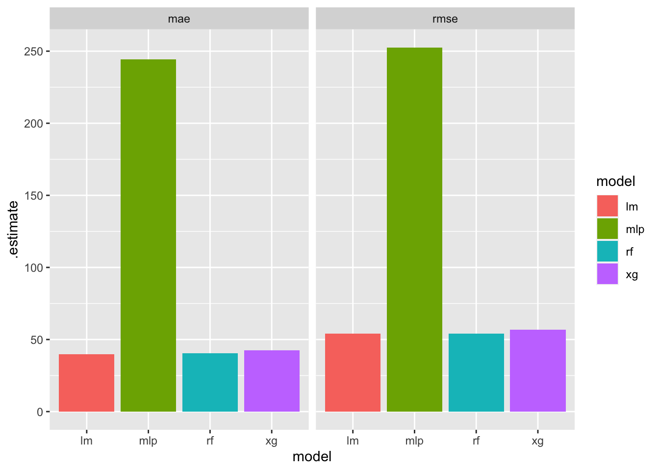
Based on the plot, it looks like linear regression might be a bit more appropriate for this problem.
Note that in the previous plot we did not show results for different recipes. Instead, the geom_col sums the errors across the two recipes. If we wanted to show results for different recipes:
t %>% ggplot(aes(x = model,y = .estimate, fill = recipe))+geom_col(position="dodge")+facet_wrap(~.metric)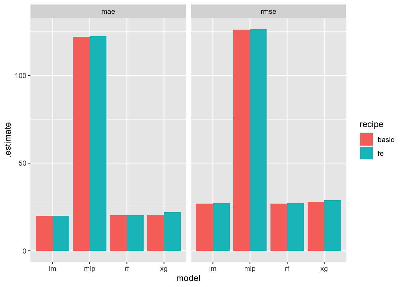
For comments, suggestions, errors, and typos, please email me at: kokkodis@bc.edu