13 Algorithmic fairness and data biases
In this chapter we will showcase how we can improve the fairness of our algorithms.
library(tidymodels)
library(tidyverse)
library(ggthemes)
set.seed(7)
13.1 Data profiling
We will use the alien income dataset. The alien income dataset includes information about an alien species’ ages, education, marital statuses, occupations, and income. Aliens can either be blue, or green. Our goal is to build an algorithm that is fair for both blue and green aliens. Hence, our objective is to build a fair algorithm in terms of alien type.
d = read_csv("../data/alien_income.csv")
d
## # A tibble: 32,561 × 7
## age workclass edu marital_status occupation alien_type income
## <dbl> <chr> <chr> <chr> <chr> <chr> <chr>
## 1 39 State-gov Bachelors Never-married Adm-cleri… green low
## 2 50 Self-emp-not-inc Bachelors Married-civ-sp… Exec-mana… green low
## 3 38 Private HS-grad Divorced Handlers-… green low
## 4 53 Private 11th Married-civ-sp… Handlers-… green low
## 5 28 Private Bachelors Married-civ-sp… Prof-spec… blue low
## 6 37 Private Masters Married-civ-sp… Exec-mana… blue low
## 7 49 Private 9th Married-spouse… Other-ser… blue low
## 8 52 Self-emp-not-inc HS-grad Married-civ-sp… Exec-mana… green high
## 9 31 Private Masters Never-married Prof-spec… blue high
## 10 42 Private Bachelors Married-civ-sp… Exec-mana… green high
## # … with 32,551 more rowsLet’s first try to do some data profiling, to see whether this data is representative of the population. The first thing is to make sure the datatypes of our data are correct. Multiple columns are of type character instead of type factor. We need to adjust these columns to factors:
d = d %>% mutate(across(c(workclass,edu,marital_status,occupation,alien_type,income), factor))Now let’s see if this dataset is representative across different types of aliens. To do so, we will tabulate our dependent variable with our variable of interest to see whether our data is representative across blue/green aliens with high/low income. The function table allows us to do so, and by dividing with the total number of instances in the dataset we can get percentages of each group:
d %>% select(income,alien_type) %>% table/nrow(d)## alien_type
## income blue green
## high 0.03620896 0.20460060
## low 0.29458555 0.46460490
13.2 Feature engineering
For now, let’s put aside the fact that this dataset is biased against blue aliens and let’s just move on with our modeling to see what kind of results we will get. To reiterate, our goal here is to predict the income of an alien given a series of observed characteristics, such as education, marital status, and so on. Our dependent variable is whether or not an alien has a high income. So we will start with our typical data splitting and recipe creation:
splits = initial_split(d, prop = 4/5)
trs = training(splits)
ts = testing(splits)
Next I am creating two recipes: one that includes the alien type, and one that does not include it. The period “.” defines all variables in the tibble except the dependent variable. The function step_rm removes the dummy-fied alien type column.
br = recipe (income ~ ., trs) %>% step_dummy(all_nominal(),-all_outcomes())
br_no_alient_type  = br %>% step_rm(alien_type_green)
br_no_alient_type %>% prep %>%  juice
## # A tibble: 26,048 × 45
## age income workclass_Federal.gov workclass_Local.gov workclass_Never.worked
## <dbl> <fct> <dbl> <dbl> <dbl>
## 1 28 low 0 1 0
## 2 38 low 0 0 0
## 3 32 low 0 0 0
## 4 34 high 0 0 0
## 5 41 low 0 0 0
## 6 37 low 0 0 0
## 7 53 low 0 0 0
## 8 41 low 0 0 0
## 9 29 low 0 0 0
## 10 26 low 0 0 0
## # … with 26,038 more rows, and 40 more variables: workclass_Private <dbl>,
## # workclass_Self.emp.inc <dbl>, workclass_Self.emp.not.inc <dbl>,
## # workclass_State.gov <dbl>, workclass_Without.pay <dbl>, edu_X11th <dbl>,
## # edu_X12th <dbl>, edu_X1st.4th <dbl>, edu_X5th.6th <dbl>,
## # edu_X7th.8th <dbl>, edu_X9th <dbl>, edu_Assoc.acdm <dbl>,
## # edu_Assoc.voc <dbl>, edu_Bachelors <dbl>, edu_Doctorate <dbl>,
## # edu_HS.grad <dbl>, edu_Masters <dbl>, edu_Preschool <dbl>, …13.3 Model definition and training
We will use two models: random forest and logistic regression. Note that since our dependent variable is binary (high or low income), this is a classification problem.
rf_class = rand_forest() %>% set_engine("ranger") %>% set_mode("classification")
lr_class = logistic_reg() %>% set_engine("glm")
bw = workflow() %>% add_model(lr_class) %>% add_recipe(br)Let’s get the predictions of each model and recipe, along with two columns of the test set: our dependent variable income, and our variable of interest alien_type.
logitPreds = bw %>%
  fit(trs) %>% predict(ts) %>% bind_cols(ts %>% select(income, alien_type))
rfPreds = bw %>% update_model(rf_class) %>%
  fit(trs) %>% predict(ts) %>% bind_cols(ts %>% select(income, alien_type))
rfPredsNA = bw %>% update_model(rf_class) %>% update_recipe(br_no_alient_type) %>%
  fit(trs) %>% predict(ts) %>% bind_cols(ts %>% select(income, alien_type))
logitPredsNA = bw %>% update_recipe(br_no_alient_type) %>%
  fit(trs) %>% predict(ts) %>% bind_cols(ts %>% select(income, alien_type))
13.4 Measuring bias
Now that we have our predictions, how can we define a measure for alien bias? One we way to do this, is to look at specificity and sensitivity. Let’s focus on sensitivity. Sensitivity is the number of true positives over the number of positives. A positive in our case is whether an individual has a high income. Hence, if the sensitivity among green aliens is higher than the sensitivity among blue aliens, then our algorithm discriminates against blue aliens.
First, let’s see if our focal event (income = 'high') is first or second (this is to figure out the event_level parameter):
levels(d$income)## [1] "high" "low"“high” appears first, so we will set event_level = "first". To get only the sensitivity score we can use the function sens from the package yardstick.
Furthermore, to get the sensitivity for each different group of aliens, we will group our predictions by alien type. The code below does that for each one of our four models:
l1 = logitPreds %>% group_by(alien_type) %>%
  sens(income,.pred_class, event_level = "first") %>%
  mutate(model = "logit", recipe = "all")
l2 = rfPreds %>% group_by(alien_type) %>%
  sens(income,.pred_class, event_level = "first") %>%
  mutate(model = "rf", recipe = "all")
l3 = rfPredsNA %>% group_by(alien_type) %>%
  sens(income,.pred_class, event_level = "first") %>%
  mutate(model = "rf", recipe="no alien type")
l4 = logitPredsNA %>% group_by(alien_type) %>%
  sens(income,.pred_class, event_level = "first") %>%
  mutate(model = "logit", recipe="no alien type")
l = bind_rows(l1,l2,l3,l4)
l
## # A tibble: 8 × 6
## alien_type .metric .estimator .estimate model recipe
## <fct> <chr> <chr> <dbl> <chr> <chr>
## 1 blue sens binary 0.335 logit all
## 2 green sens binary 0.585 logit all
## 3 blue sens binary 0.425 rf all
## 4 green sens binary 0.589 rf all
## 5 blue sens binary 0.430 rf no alien type
## 6 green sens binary 0.578 rf no alien type
## 7 blue sens binary 0.376 logit no alien type
## 8 green sens binary 0.576 logit no alien typeTo understand the results, let’s focus on the first two rows: the logistic regression model predicts only ~33% of the blue aliens who have high income. On the other hand, the same algorithm, predicts ~59% of the green aliens who have high income. In other words, the algorithm discriminates against blue aliens by identifying a significantly smaller percentage of the high income ones.
Let’s plot these results to get a better idea:
l %>% ggplot(aes(x=alien_type, y =.estimate, fill = model)) +
  geom_col(position = "dodge") +facet_wrap(~recipe)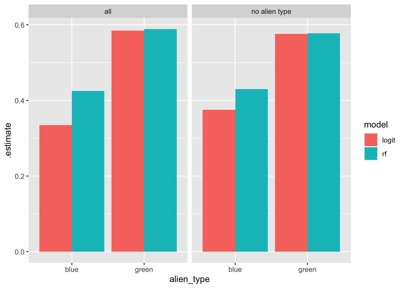
From this plot it becomes clear: Both algorithms, independent of whether or not we include alien type in our recipes, disproportionately penalize blue aliens by systematically identifying proportionally fewer blue aliens from those who have high income. Note that as data analysts, we did nothing wrong. Also note that the algorithms themselves, do not know what an alien type is and how to discriminate against blue aliens. The algorithms have their own mathematical objectives that they want to meet. It just happens that because the input data is not representative, the algorithms end up learning models that are inherently biased.
13.5 Debiasing results
Now let’s pick one model to try to de-bias. Let’s first estimate the AUC score. We will use the evalClass function from the Section 11.4.3:
evalClass = function(aWorkFlow){
  tmpFit = aWorkFlow %>% fit(trs)
  p = predict(tmpFit, ts, "prob") %>%  bind_cols(ts %>% select(income))
  p %>% roc_auc(truth = income, .pred_high, event_level = "first")
}
bw %>% evalClass## # A tibble: 1 × 3
## .metric .estimator .estimate
## <chr> <chr> <dbl>
## 1 roc_auc binary 0.885bw %>% update_model(rf_class) %>% evalClass## # A tibble: 1 × 3
## .metric .estimator .estimate
## <chr> <chr> <dbl>
## 1 roc_auc binary 0.892Let’s now get the probability predictions.
probs = bw %>% update_model(rf_class) %>% fit(trs) %>% predict(ts,"prob") %>%
   bind_cols(ts %>% select(income, alien_type))
Next, we will create a function that takes as input a threshold, and based on that threshold, it estimates the sensitivity for blue and green aliens. The only new piece of code in this function is the threshold usage that creates custom labels (customLabels column):
getRatio = function(thr){
  tmp = probs %>% mutate(customLabels = factor(ifelse(.pred_high > thr, "high","low"), levels = c("high","low")))
  acc = tmp %>% accuracy(income,customLabels)
  tmp = tmp %>%  group_by(alien_type) %>% sens(income,customLabels, event_level = "first")
  # here i am dividing the sensitivity of green aliens
  # over the sensitivity of blue aliens to quantify the level
  # of bias against blue aliens.
  f = (tmp[2,4]/tmp[1,4]) %>% rename(ratio = .estimate) %>% mutate(acc = acc$.estimate, thr = thr)
  return(f)
}
Let’s now test multiple thresholds:
f = seq(0.1,0.8,0.05) %>% map_dfr(getRatio)
f
## ratio acc thr
## 1 1.058766 0.6433287 0.10
## 2 1.105528 0.7062797 0.15
## 3 1.141145 0.7486565 0.20
## 4 1.233092 0.7761400 0.25
## 5 1.292179 0.8007063 0.30
## 6 1.295405 0.8209734 0.35
## 7 1.230512 0.8338707 0.40
## 8 1.312546 0.8381698 0.45
## 9 1.426132 0.8375557 0.50
## 10 1.585994 0.8358667 0.55
## 11 1.773089 0.8321818 0.60
## 12 2.418836 0.8249655 0.65
## 13 3.454069 0.8123752 0.70
## 14 7.519797 0.7970213 0.75
## 15 Inf 0.7776754 0.80Let’s plot the results along with the accuracy score of each threshold, to see if we can pick a threshold that minimizes bias while maintaining a high level of accuracy. The function pivot_longer here is the opposite of pivot_wider: it takes multiple columns and puts their values under two columns, one that identifies the original column name (parameter names_to) and one that identifies the value (parameter values_to):
f %>% pivot_longer(-thr, names_to = "metric", values_to = "score") %>%
  ggplot(aes(x=thr, y = score, color = metric)) + geom_point()+
  theme_fivethirtyeight()+geom_line() + ylim(c(0,1.5))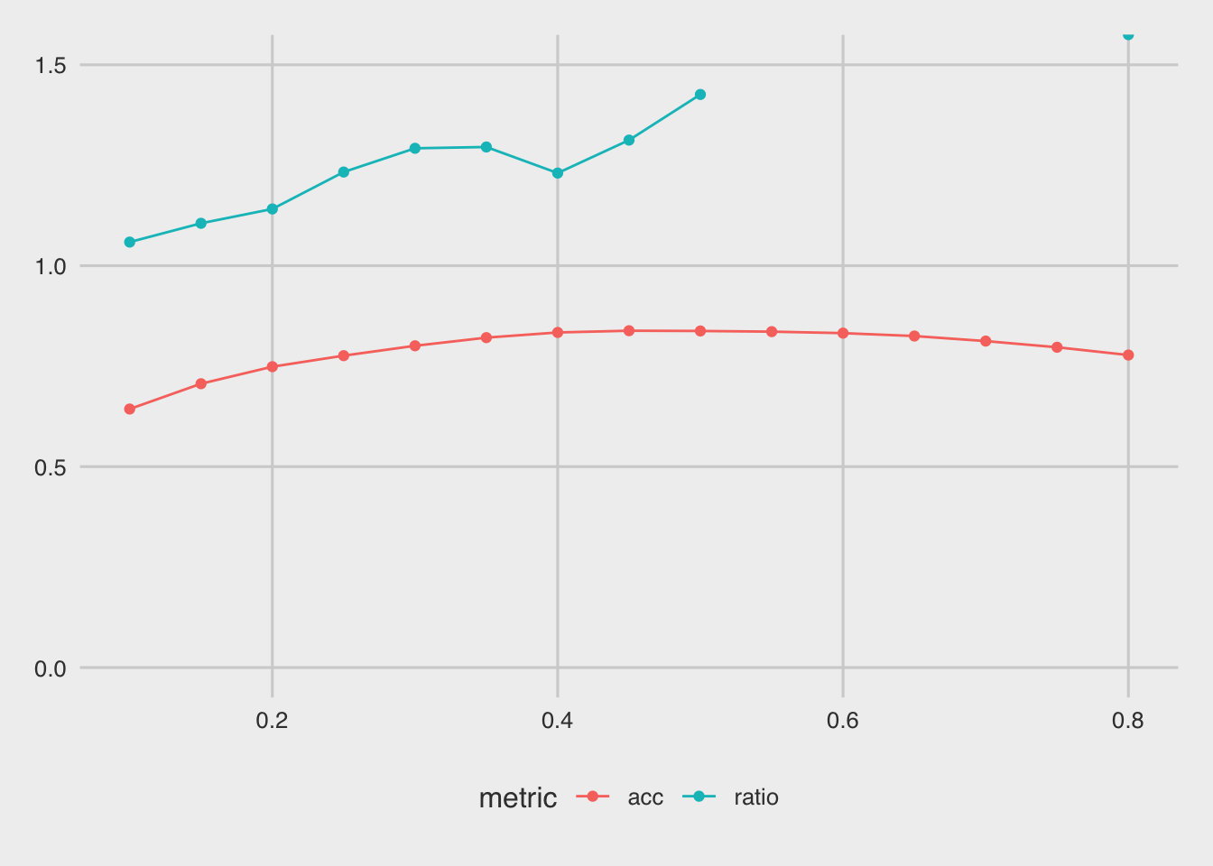
Based on this plot, a threshold around 0.1 seems to minimize the bias, however it also hurts the accuracy of the model:
getRatio(0.1)## ratio acc thr
## 1 1.058766 0.6433287 0.1Let’s see the sensitivity of blue and green aliens for threshold = 0.1:
thr = 0.1
tmp = probs %>% mutate(customLabels = factor(ifelse(.pred_high > thr, "high","low"), levels = c("high","low")))
tmp = tmp %>%  group_by(alien_type) %>% sens(income,customLabels, event_level = "first")
tmp
## # A tibble: 2 × 4
## alien_type .metric .estimator .estimate
## <fct> <chr> <chr> <dbl>
## 1 blue sens binary 0.919
## 2 green sens binary 0.973As you can see, the two sensitivity scores are now much much closer than in the default state of the algorithm.
Recall that by default algorithms use a probability threshold = 0.5.
For comments, suggestions, errors, and typos, please email me at: kokkodis@bc.edu