5 Collecting structured data from the Web

In this and the following chapter we will use four new packages: * httr handles API calls. * rtweet which is an R package for efficient use of the Twitter API. * tidyquant which focuses on financial analysis. * rvest which allows us to scrape HTML web pages.

We will first install these packages (only once):

install.packages(c("httr","rtweet","tidyquant","rvest"))

Then we will load them into our environment as follows:

library(tidyverse)
library(httr)
library(jsonlite)
library(rtweet)
library(tidyquant)
library(lubridate)

We will first collect structured output from Application Programming Interfaces (APIs).

5.1 Simple API calls: dog-facts

We will starts by using the package httr to make simple API calls. httr allows us to retrieve and post information from specific URLs (AKA endpoints). It has two basic functions: the GET() function that retrieves information from a given URL, and the POST() function that transfers information to a given URL.

As an example, we will use the dog-facts API (https://dukengn.github.io/Dog-facts-API/):

APIs and webpages dynamically change over time. As a result, some of these examples might not work as presented.

 

r = GET("https://dog-facts-api.herokuapp.com/api/v1/resources/dogs/all")

One way to access the information of any R object, is to call the function names():

names(r)

By running names(r) we observe that there is a field content. This field stores the response of the API call in binary format. We can access any field of an R object with the dollar sign $ as follows:

# Run r$content in your machine to see the results. 
# I omit the output here for presentation purposes. 
r$content

Recall that the dollar sign $ can also be used to access any column c from a tibble t (t$c).

As humans, we can’t really work with binary code; to encode and translate this binary response we can use the rawToChar() function and get the result as a JSON object:

j = rawToChar(r$content)

The results are in JSON format because this is how the specific API formats its responses. Most APIs return JSON objects, but some might occassionaly return different formats (e.g., CSV or XML).

Now we can call the function fromJSON() from package jsonlite (see Section 4.2) that immediately transforms a JSON object into a data frame:

t = fromJSON(rawToChar(r$content))

Recall that a data frame behaves almost identical to a tibble. Yet, for consistency, we can use the function as_tibble to transform its internal representation into a tibble. Combining with the code from the previous chunk:

t = as_tibble(fromJSON(rawToChar(r$content)))

Now we have a final clean tibble that we can explore and manipulate as we discusses earlier in Section 2.3.

5.2 API calls with parameters

Besides getting all available information from an API endpoint, we often need to specify the chunks of information that we are interested in.

To show an example we will use the COVID-19 API that allows us to get live stats on COVID infections, recoveries, and deaths, per country. The API’s documentation can be found here: https://documenter.getpostman.com/view/10808728/SzS8rjbc (Main website: https://covid19api.com)

Assume that we want to get the confirmed cases in the Greece, between June 1st and August 26th. To do so, we add after the endpoint a question mark ?, followed by the parameters that define the period we are looking for:

r = GET("https://api.covid19api.com/country/greece/status/confirmed?from=2021-06-01T00:00:00Z&to=2021-08-26T00:00:00Z")
r

## Response [https://api.covid19api.com/country/greece/status/confirmed?from=2021-06-01T00:00:00Z&to=2021-08-26T00:00:00Z]
##   Date: 2021-10-26 00:08
##   Status: 200
##   Content-Type: application/json; charset=UTF-8
##   Size: 15 kB
## [{"Country":"Greece","CountryCode":"GR","Province":"","City":"","CityCode":""...

Similar to before, we transform the result to a tibble:

r1 =  as_tibble(fromJSON(rawToChar(r$content)))
r1 %>%  head

## # A tibble: 6 × 10
##   Country CountryCode Province City  CityCode Lat   Lon    Cases Status  Date   
##   <chr>   <chr>       <chr>    <chr> <chr>    <chr> <chr>  <int> <chr>   <chr>  
## 1 Greece  GR          ""       ""    ""       39.07 21.82 404163 confir… 2021-0…
## 2 Greece  GR          ""       ""    ""       39.07 21.82 405542 confir… 2021-0…
## 3 Greece  GR          ""       ""    ""       39.07 21.82 406751 confir… 2021-0…
## 4 Greece  GR          ""       ""    ""       39.07 21.82 407857 confir… 2021-0…
## 5 Greece  GR          ""       ""    ""       39.07 21.82 408789 confir… 2021-0…
## 6 Greece  GR          ""       ""    ""       39.07 21.82 409368 confir… 2021-0…

5.2.1 Handling dates

If we examine the resulting tibble, we can see that there is a column named Date. However R thinks that this is character (<chr>) column. Fortunately, we can transform this column to a date type with the function as_date() from the package lubridate:

r1$Date = as_date(r1$Date)
r1 %>%  head

## # A tibble: 6 × 10
##   Country CountryCode Province City  CityCode Lat   Lon    Cases Status   
##   <chr>   <chr>       <chr>    <chr> <chr>    <chr> <chr>  <int> <chr>    
## 1 Greece  GR          ""       ""    ""       39.07 21.82 404163 confirmed
## 2 Greece  GR          ""       ""    ""       39.07 21.82 405542 confirmed
## 3 Greece  GR          ""       ""    ""       39.07 21.82 406751 confirmed
## 4 Greece  GR          ""       ""    ""       39.07 21.82 407857 confirmed
## 5 Greece  GR          ""       ""    ""       39.07 21.82 408789 confirmed
## 6 Greece  GR          ""       ""    ""       39.07 21.82 409368 confirmed
## # … with 1 more variable: Date <date>

Note that we have already loaded the package lubridate in our working environment in the begining.

Once we transform the column into a date type, we can use date-specific functions from the package lubridate that can manipulate dates. For instance, we can use the function wday() which will return the day of the week for each date:

wday(r1$Date, label = T) %>% head

## [1] Tue Wed Thu Fri Sat Sun
## Levels: Sun < Mon < Tue < Wed < Thu < Fri < Sat

In the previous call of wday we set label = T. This argument returns the results in labels (such as Fri, Sat, Sun, Mon, etc.). Experiment with running wday() with label = F to see the difference.

For more information on the available functions of lubridate, you can use this cheatsheet: https://lubridate.tidyverse.org

 

5.2.2 Data analysis of data collected from an API

Let us assume now that we want to estimate the number of confirmed cases per weekday. First, we need to create a weekday column that stores the day of the week:

r2 = r1 %>% mutate(weekday = wday(Date, label=T))
r2 %>% head

## # A tibble: 6 × 11
##   Country CountryCode Province City  CityCode Lat   Lon    Cases Status   
##   <chr>   <chr>       <chr>    <chr> <chr>    <chr> <chr>  <int> <chr>    
## 1 Greece  GR          ""       ""    ""       39.07 21.82 404163 confirmed
## 2 Greece  GR          ""       ""    ""       39.07 21.82 405542 confirmed
## 3 Greece  GR          ""       ""    ""       39.07 21.82 406751 confirmed
## 4 Greece  GR          ""       ""    ""       39.07 21.82 407857 confirmed
## 5 Greece  GR          ""       ""    ""       39.07 21.82 408789 confirmed
## 6 Greece  GR          ""       ""    ""       39.07 21.82 409368 confirmed
## # … with 2 more variables: Date <date>, weekday <ord>

Now if we look at the data, the API provides commutative numbers of confirmed cases in each area. So in order to get the new number of confirmed cases per day, we will need to subtract from each day the number of confirmed cases from the previous day.

R has a function lag() that takes as input a variable and shifts the variable one time period so that each observation stores the value of the previous period. This is particularly useful in time series data.

Note that for lag() to work properly the tibble must be ordered. In this example, it is already ordered by the API response.

You can find more info about the lag() function here: https://dplyr.tidyverse.org/reference/lead-lag.html

 

As an example, check out the first six values of the original Cases column:

r2 = r1
r2$Cases %>%  head

## [1] 404163 405542 406751 407857 408789 409368

Now see how the lag() function shifts those values:

lag(r2$Cases) %>%  head

## [1]     NA 404163 405542 406751 407857 408789

With lag() we can estimate the numberOfNewCases for each day by subtracting the number of previous cases stored in the lagged variable. Then, we can group by the new column weekday to estimate the average number of new cases per weekday:

r1 %>%  mutate(weekday = wday(Date, label=T), numberOfNewCases = Cases - lag(Cases)) %>% 
        select(Cases,weekday,numberOfNewCases) %>% group_by(weekday) %>% 
        summarize(averageCases = mean(numberOfNewCases, na.rm = T))

## # A tibble: 7 × 2
##   weekday averageCases
##   <ord>          <dbl>
## 1 Sun            1153.
## 2 Mon            1531.
## 3 Tue            2975.
## 4 Wed            2121.
## 5 Thu            2077.
## 6 Fri            2008.
## 7 Sat            1905.

Alternatively, we can plot the number of new cases over time:

r1 %>%   mutate(weekday = wday(Date, label=T),numberOfNewCases = Cases - lag(Cases)) %>% 
   ggplot(aes(x=Date, y=numberOfNewCases))+geom_line()+geom_smooth()+theme_tufte()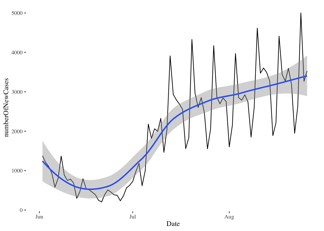

Note that ggplot knows how to use the Date column as a date: it automatically transforms the date values into Jun, Jul, and Aug.

5.3 Authentication with the Twitter API wrapper rtweet

Not every API is open for everyone to query. Some APIs require authentication. Take for instance the Twitter API. In order to gain access to Twitter data, we first need to have a Twitter account, and submit an application that explains the reasons that we want to use the Twitter API. You can find more info here: https://developer.twitter.com/en/docs

For the ISYS 3350 students, I have provided you the necessary credentials to access the Twitter API. As a result, you do not need to submit an application.

Instead of using the GET() function to access the Twitter API, we will use the package rtweet which is an API wrapper. API wrappers are language-specific packages that wrap API calls into easy-to-use functions. So instead of using every time the function GET with a specific endpoint, wrappers include functions that encapsulate these end points and streamline the communication between our program and the API.

You can find more info about the rtweet wrapper` here:https://github.com/ropensci/rtweet

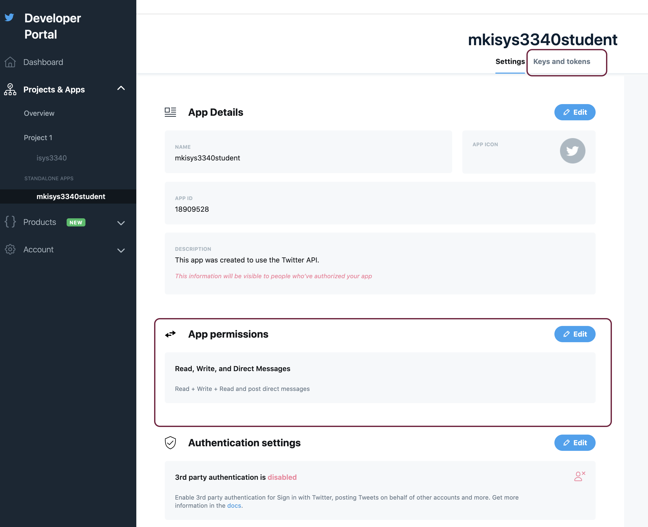
5.3.1 create_token()

The first thing we will do in order to use the wrapper rtweet is to create a unique signature that allows us to completely control and manipulate our twitter account. We will need the key, secret key, access token, secret access token, and the application name. We can get this info from our developer twitter account (keys and tokens section).

Then, we can store these keys into variables as follows:

key = "replaceWithYourKey"
secret = "replaceWithYourSecret"
access = "replaceWithYourAccessKey"
access_secret = "replaceWithYourAccessSecret"
app_name = "replaceWithYourAppName"

Attention: These keys are not valid and will not work. You will need to generate and use your own keys.

Once we have the necessary keys, we can use the function create_token() to generate our unique signature.

myToken = create_token(app = app_name,
             consumer_key = key, 
             consumer_secret = secret,
             access_token = access,
             access_secret = access_secret)

5.3.2 post_tweet()

Now we can use our signature along with the function post_tweet to post a new tweet:

post_tweet("The students of ISYS3340  are the best! Period.", token = myToken)

5.3.3 search_tweets()

We can use the function search_tweets() to look for specific tweets, for instance, tweets that include the hashtag #analytics:

analytics = search_tweets("#analytics", n=50,token = myToken, 
                          include_rts = F)
analytics %>% head

## # A tibble: 6 × 90
##   user_id    status_id           created_at          screen_name  text    source
##   <chr>      <chr>               <dttm>              <chr>        <chr>   <chr> 
## 1 3219670842 1452788912892497920 2021-10-26 00:07:23 njoyflyfish… 7 Day … smcap…
## 2 3219670842 1452782032971460622 2021-10-25 23:40:02 njoyflyfish… 7 Day … smcap…
## 3 3219670842 1452788285655314435 2021-10-26 00:04:53 njoyflyfish… 7 Day … smcap…
## 4 3219670842 1452787759249125376 2021-10-26 00:02:47 njoyflyfish… 7 Day … smcap…
## 5 3219670842 1452784188134871040 2021-10-25 23:48:36 njoyflyfish… 7 Day … smcap…
## 6 3219670842 1452777830320795649 2021-10-25 23:23:20 njoyflyfish… 7 Day … smcap…
## # … with 84 more variables: display_text_width <dbl>, reply_to_status_id <lgl>,
## #   reply_to_user_id <lgl>, reply_to_screen_name <lgl>, is_quote <lgl>,
## #   is_retweet <lgl>, favorite_count <int>, retweet_count <int>,
## #   quote_count <int>, reply_count <int>, hashtags <list>, symbols <list>,
## #   urls_url <list>, urls_t.co <list>, urls_expanded_url <list>,
## #   media_url <list>, media_t.co <list>, media_expanded_url <list>,
## #   media_type <list>, ext_media_url <list>, ext_media_t.co <list>, …

Note that you can increase the argument n=50 to fetch more tweets. The argument include_rts=F tells rtweet to not return retweets.

5.4 tidyquant

A different wrapper that focuses on financial markets is the tidyquant wrapper. This is a package that facilitates financial analysis, as it focuses on providing the tools to perform stock portfolio analysis at scale.

You can find a lot of information here:https://cran.r-project.org/web/packages/tidyquant/vignettes/TQ00-introduction-to-tidyquant.html

 

For our example, we want to plot the stock prices for “AAPL”,‘TSLA’, and ‘ZM’, for 9 months, between January 2021 and September 2021. The function tq_get() returns quantitative data in tibble format:

r = c("AAPL",'TSLA','ZM') %>% tq_get(get = "stock.prices",
                                 from = "2021-01-01",
                                 to = "2021-09-01")

## Warning: `type_convert()` only converts columns of type 'character'.
## - `df` has no columns of type 'character'

## Warning: `type_convert()` only converts columns of type 'character'.
## - `df` has no columns of type 'character'

## Warning: `type_convert()` only converts columns of type 'character'.
## - `df` has no columns of type 'character'

r %>% head

## # A tibble: 6 × 8
##   symbol date        open  high   low close    volume adjusted
##   <chr>  <date>     <dbl> <dbl> <dbl> <dbl>     <dbl>    <dbl>
## 1 AAPL   2021-01-04  134.  134.  127.  129. 143301900     129.
## 2 AAPL   2021-01-05  129.  132.  128.  131.  97664900     130.
## 3 AAPL   2021-01-06  128.  131.  126.  127. 155088000     126.
## 4 AAPL   2021-01-07  128.  132.  128.  131. 109578200     130.
## 5 AAPL   2021-01-08  132.  133.  130.  132. 105158200     131.
## 6 AAPL   2021-01-11  129.  130.  128.  129. 100384500     128.

Now we can plot the results:

r %>% ggplot(aes(y=adjusted, x=date, color = symbol, fill = symbol)) + 
  geom_smooth()+theme_economist()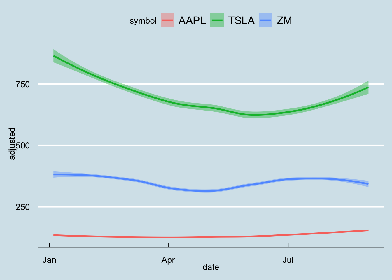

---

For comments, suggestions, errors, and typos, please email me at: kokkodis@bc.edu