1 Introduction to R and tidyverse
1.1 Introduction to R Markdown
When we write code, we often want to be able to make changes and re-use it. To facilitate this process, R allows us to create files that store our code. R Markdown files allow us to insert chunks of R code.
To create an R Markdown file, click on
File\(\rightarrow\)New File\(\rightarrow\)R Markdown.... ClickOKand then save this markdown file in yourRmddirectory. us_r
In your R Markdown file, open a chunk by typing three left quotes, followed by the letter r inside curly brackets (```{r}); Close the chunk by typing three left quotes ```. Anything inside an R chunk is interpreted as R code.
Cmd + Option + I (Mac) or
Ctrl + Alt + I (Windows)
1.1.1 Running chunks
To run an R chunk click on the green button at the end of the first line inside the chunk:
Or click:
- Cmd + Shift + Enter (Mac)
- Control + Shift + Enter (Windows)
To execute the code of a single line inside an R chunk you can click:
- Cmd + Enter (Mac)
- Control + Enter (Windows)
The results of the R chunk are also printed out in the console.
1.1.2 A basic example
Insert a new R chunk, and then type the following:
5+5
4+10
4-9
## [1] 10
## [1] 14
## [1] -5Run the chunk to see the results.
1.2 Variables in R
In programming, variables are essentially nicknames that we use to store values or other language objects. For example, let us say that we want to store a person’s age in a variable. We can create a new variable and name it “age.” Then, we can store the appropriate age value to this variable.
In R, we store values to variables by using the symbol = (or <-, ->).
The name of a variable can be any sequence of characters given that it starts with a letter.
Variable names are case sensitive.
age=36 # A hashtag inside an R chunk creates a comment.
        # R knows to ignore comments (comments are explanations for humans)
age<-36 # age is a variable that stores the number 36
Other variable names that can store the number 36:
x <- 36 # x is a variable that also stores the number 36
age36 <- 36 #age36  is a variable that stores the number 36
z1 <- 36 # z1 is a variable that stores the number 36
Choose variable names that best represent the stored values.
1.3 Vectors
In R, lowercase c followed by a parenthesis is a special keyword that identifies a vector. A vector is a sequence of data elements. Below, the variable quiz_results is a vector that stores the scores of a hypothetical quiz.
quiz_results = c(9,8,4,10)
quiz_results
## [1] 9 8 4 10Note that by just typing the name of a variable (in our example
quiz_results) inside an R chunk and running it R prints out the value(s) of that variable.
Elements in a vector can be accessed by their position. For example, in our vector quiz_results:
- 9 \(\rightarrow\) \(1^{st}\) position
- 8 \(\rightarrow\) \(2^{nd}\) position
- 4 \(\rightarrow\) \(3^{rd}\) position
- 10 \(\rightarrow\) \(4^{th}\) position
Hence, we can access the element in the \(2^{nd}\) position as follows:
quiz_results[2]## [1] 8And we can assign it to a new variable:
second_element = quiz_results[2]
second_element
## [1] 81.4 Data types
In programming (and in R) each variable has a data type, which describes what kind of information the variable stores. For instance, in our previous example, variable age is a numeric variable, because it stores a numeric value.
R allows us to define variables that are not numeric. For example, we can create a variable that is a sequence of characters. Consider a variable that stores the word “data.” We can name this variable data_var and assign to it the characters data.
data_var <- 'data'
data_var
## [1] "data"Any sequence of characters in single (') or double (") quotes is considered a string. For instance, the following line of code that uses double quotes has the same result:
data_var <- "data"
data_var
## [1] "data"Variables that store strings are of data type
character.
R allows for other types of variables, such as date variables and factors. We will introduce these types of variables later in the class.
If our variables are of data type numeric, we can add, subtract, divide, and multiply them as follows:
x = 7
y = 13
x + y
x - y
x / y
x * y
## [1] 20
## [1] -6
## [1] 0.5384615
## [1] 911.5 Functions in R
A function is a stored, pre-defined block of code that operates on some input value to return an output.
R has multiple built-in functions that we can apply to our variables.
For instance, the function log() will estimate the logarithm of its input:
log(age)## [1] 3.583519In the above, age is the input of the function log, and the output of the function is the logarithm of variable age. Of course we can also apply the function log to a number:
log(36)## [1] 3.583519Similarly, the function sqrt() estimates the square root of a numeric variable (or a number):
sqrt(x)
sqrt(10)
## [1] 2.645751
## [1] 3.162278The input of a function does not need to be a scalar (one-element) variable; functions can also operate on vectors (and other structures that we will learn in the future).
Since we have a vector of quiz results, it would be nice to know what was the average quiz performance. We can call the function mean() on the vector quiz_results:
meanQuiz = mean(quiz_results)
meanQuiz
## [1] 7.75Similarly, we can estimate the standard deviation of the quiz results with the function sd:
sdQuiz = sd(quiz_results)
sdQuiz
## [1] 2.629956Since we have already estimated the mean and the standard deviation of the vector quiz_results,
we can also standardize it by subtracting the mean and dividing with the standard deviation.
standardQuiz <- (quiz_results - meanQuiz)/sdQuiz
quiz_results
standardQuiz
## [1] 9 8 4 10
## [1] 0.47529319 0.09505864 -1.42587956 0.85552774By standardizing the quiz results we created a new vector standardQuiz which has a zero mean and standard deviation of 1.
mean(standardQuiz)
sd(standardQuiz)
## [1] 1.734723e-17
## [1] 1We can plot and compare the histograms of the two vectors with the function hist:
hist(quiz_results,main = "") # the option main = "" removes the title from the figure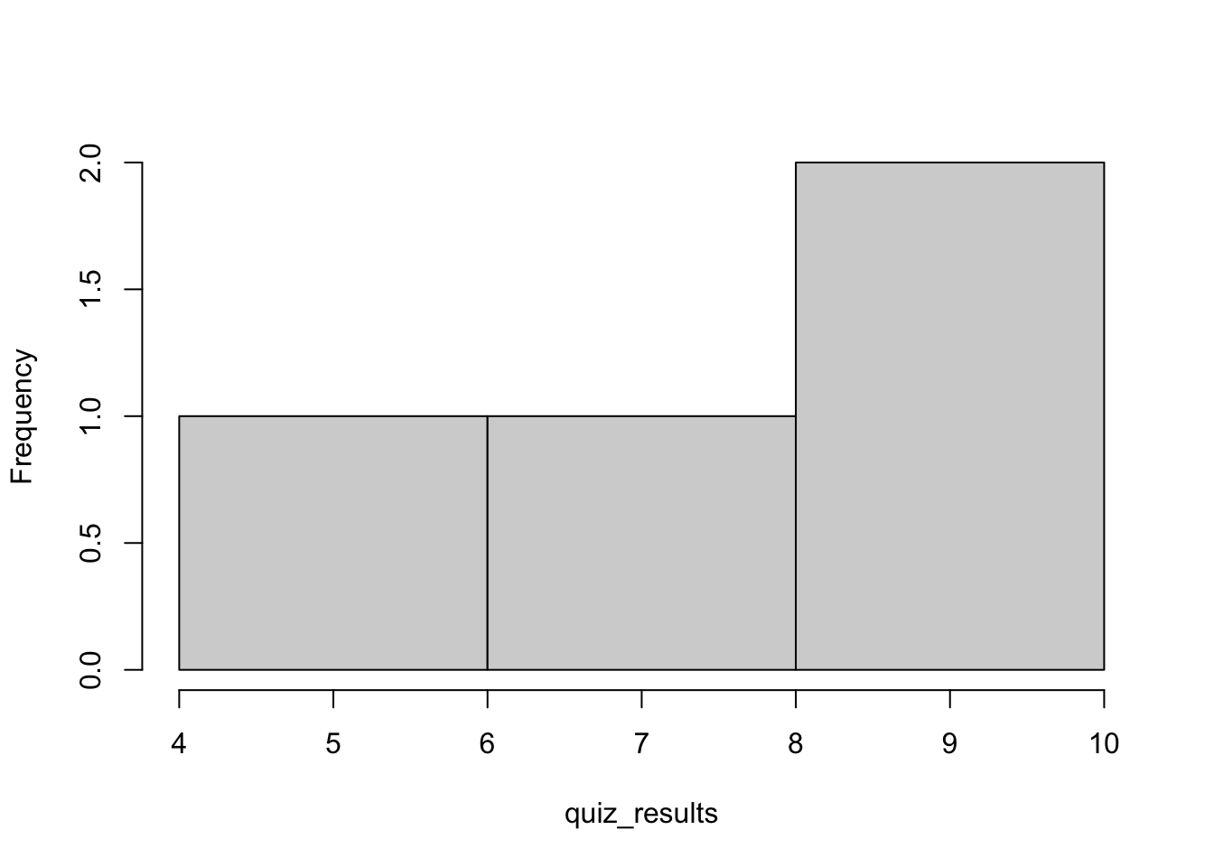
Figure 1.1: Histogram of the original vector
hist(standardQuiz, main = "")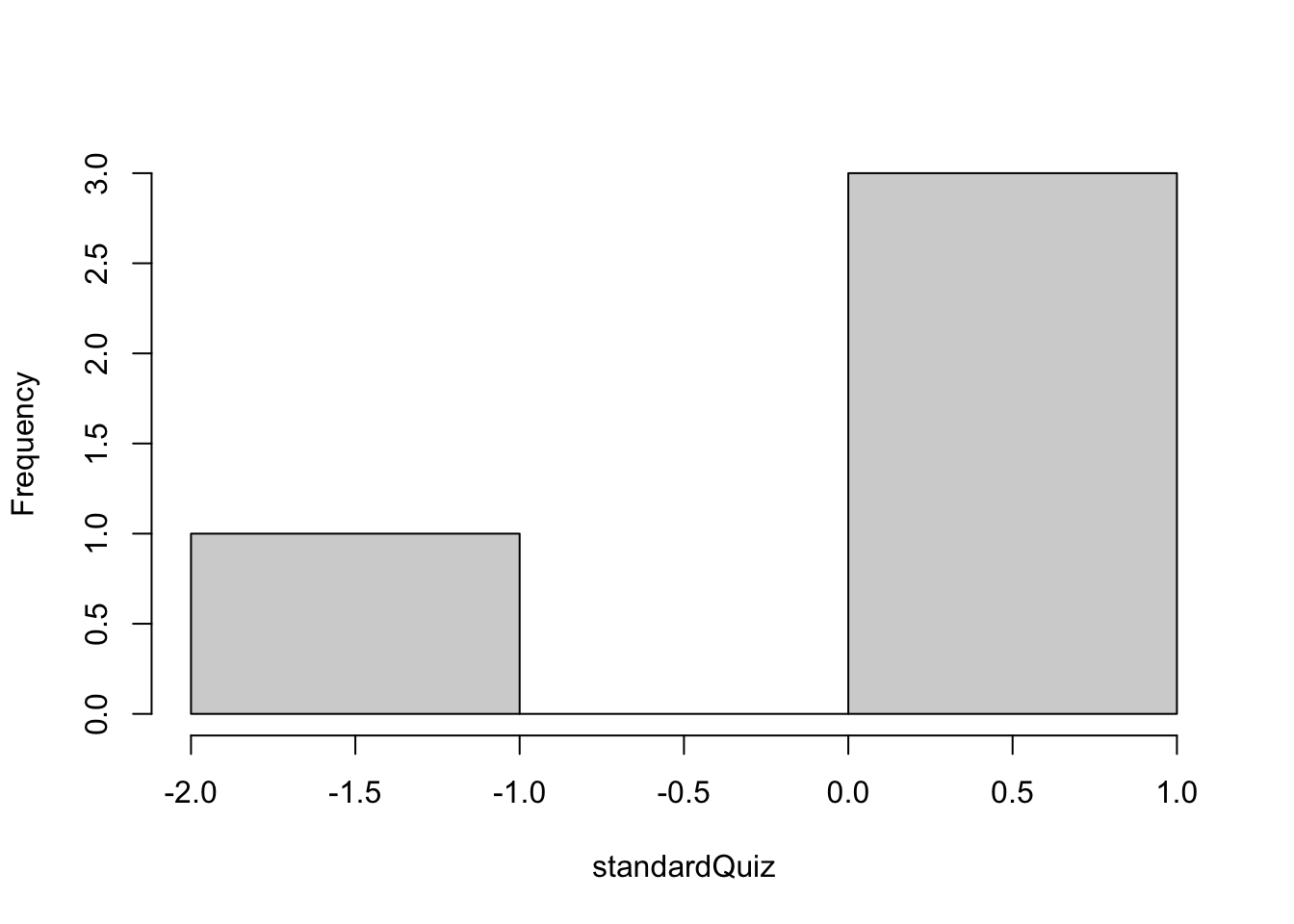
Figure 1.2: Histogram of the standardized vector
When calling the function
hist()in the previous two examples we used two inputs: the first input was the vector name (quiz_resultsorstandardQuiz); the second input was the empty string"", which told functionhist()to not print a title for the figure. In general, a function can take as input multiple variables.
You can experiment with the above code by changing the empty quote to a string, for instance, main="what a great histogram".
standardQuiz in hist(standardQuiz, main = "") is an argument.)
main in hist(standardQuiz, main = "") is a parameter.)
1.6 Logic
Besides numeric and character variables we can also have logical variables.
A logical variable can either be TRUE or FALSE. (TRUE and FALSE are special keywords in R).
We can also use the letters
TandFto indicateTRUEandFALSErespectively.
x = F #FALSE, assign the logical value FALSE to variable x
y = T #TRUE, assign the logical value True to variable x
x
## [1] FALSEy## [1] TRUE1.6.1 Logical operators
With logical variables we can use logical operators. A logical operator is a way to make a test in R. R supports the following logical operators:
| Operator | Description |
|---|---|
| < | Less than |
| <= | Less than or equal to |
| > | Greater than |
| >= | Greater than or equal to |
| == | Exactly equal to |
| ! | Not (negation) |
| & | Logical AND |
| | | Logical OR |
A logical AND compares two statements. If both statements are
TRUEthen the result of the comparison is alsoTRUE; Otherwise the result of the comparison isFALSE
Here is the truth table of logical AND:
| X | Y | X AND Y |
|---|---|---|
| TRUE | TRUE | TRUE |
| TRUE | FALSE | FALSE |
| FALSE | TRUE | FALSE |
| FALSE | FALSE | FALSE |
A logical OR compares two statements. If either or both of the statements are
TRUEthen the result of the comparison isTRUE; Otherwise, if both statements areFALSEthe result of the comparison isFALSE.
| X | Y | X OR Y |
|---|---|---|
| TRUE | TRUE | TRUE |
| TRUE | FALSE | TRUE |
| FALSE | TRUE | TRUE |
| FALSE | FALSE | FALSE |
Here are some examples that used the logical variables x and y from above:
x & y
x | y
!x & y
## [1] FALSE
## [1] TRUE
## [1] TRUEx = 5
y = 6
x == y
x != y
x < y
x > y## [1] FALSE
## [1] TRUE
## [1] TRUE
## [1] FALSEWe can group conditions together through parentheses:
z = 10
(x != y) & (x < z)  #Both parentheses are TRUE and hence the result is TRUE
## [1] TRUE(x != y) | (x < z) ## [1] TRUE= and a double ==: A single = assignes a value to a variable; a double == is a logical test between the left-hand side and the right-hand side.
1.6.2 The ifelse() function
A particularly interesting function in R is the ifelse() function, which allows us to apply a transformation only if a condition is TRUE. For instance, we can partially update the quiz scores (in our vector quiz_results) that are less than 9:
# return 1 for those scores that are less or equal to 8. Otherwise return 0:
ifelse(quiz_results <= 8,1,0)
## [1] 0 1 1 0Of course, we can assign the result of an ifelse() transformation to the original variable (or to a new variable):
# update scores lower than 9 with -1:
quiz_results_transformed = ifelse(quiz_results < 9,-1,quiz_results) # assign the transformed result to a new variable
quiz_results = ifelse(quiz_results < 9,-1,quiz_results) # assign the tranformed results to the original variable
quiz_results
## [1] 9 -1 -1 101.6.3 More examples of logic and logical operators
Below are some additional examples of logic and logical operators.
A = 6
B = 7
C = 10
D = T
A==B # Is A equal to B?
!(B > C) | (!D) # Not B greater than C OR not D.
# A less or equal than C AND  ( not B greater than C OR not D)
(A <= C) & (!(B > C) | (!D))
## [1] FALSE
## [1] TRUE
## [1] TRUE1.7 R Packages and summarizing a real dataset
Very often we will need to use R functions that are not already built in. In these cases, we will need to install and load R packages. These packages include code written by independent developments and teams, and it is free for everyone to use and change.
As an example, let’s install the package mlbench by calling the function install.packages as follows:
install.packages("mlbench")We can also install packages manually from RStudio:
Packages tab\(\rightarrow\)install.
mlbench from this point on unless there is an updated version of it.
To see the available datasets from the newly installed package mlbench we can call the function data and pass the argument ‘mlbench’ to the parameter package as follows:
data(package='mlbench')To make the functions and datasets of the package mlbench available to us we need to call the function library():
library(mlbench)library(package_name)
Now we can use the datasets and functions of the mlbench package. Let us load the dataset BreastCancer with function data().
data("BreastCancer")
head(BreastCancer)
## Id Cl.thickness Cell.size Cell.shape Marg.adhesion Epith.c.size
## 1 1000025 5 1 1 1 2
## 2 1002945 5 4 4 5 7
## 3 1015425 3 1 1 1 2
## 4 1016277 6 8 8 1 3
## 5 1017023 4 1 1 3 2
## 6 1017122 8 10 10 8 7
## Bare.nuclei Bl.cromatin Normal.nucleoli Mitoses Class
## 1 1 3 1 1 benign
## 2 10 3 2 1 benign
## 3 2 3 1 1 benign
## 4 4 3 7 1 benign
## 5 1 3 1 1 benign
## 6 10 9 7 1 malignantThe function
headallows us to explore the first six rows of a dataset. Similarly, the functiontailallows us to explore the last six rows of a dataset.
Now, we can get the summary statistics of this dataset with the function summary().
summary(BreastCancer)## Id Cl.thickness Cell.size Cell.shape Marg.adhesion
## Length:699 1 :145 1 :384 1 :353 1 :407
## Class :character 5 :130 10 : 67 2 : 59 2 : 58
## Mode :character 3 :108 3 : 52 10 : 58 3 : 58
## 4 : 80 2 : 45 3 : 56 10 : 55
## 10 : 69 4 : 40 4 : 44 4 : 33
## 2 : 50 5 : 30 5 : 34 8 : 25
## (Other):117 (Other): 81 (Other): 95 (Other): 63
## Epith.c.size Bare.nuclei Bl.cromatin Normal.nucleoli Mitoses
## 2 :386 1 :402 2 :166 1 :443 1 :579
## 3 : 72 10 :132 3 :165 10 : 61 2 : 35
## 4 : 48 2 : 30 1 :152 3 : 44 3 : 33
## 1 : 47 5 : 30 7 : 73 2 : 36 10 : 14
## 6 : 41 3 : 28 4 : 40 8 : 24 4 : 12
## 5 : 39 (Other): 61 5 : 34 6 : 22 7 : 9
## (Other): 66 NA's : 16 (Other): 69 (Other): 69 (Other): 17
## Class
## benign :458
## malignant:241
##
##
##
##
## We will use the functions
head,tail, andsummary()repeatedly throughout this book to get a first look at each new dataset.
1.8 tidyverse
tidyverse is a collection of R packages designed for data science. All packages share an underlying design philosophy, grammar, and data structures.
Install the tidyverse package as follows:
install.packages("tidyverse")tidyverse from this point on unless there is an updated version of it.
tidyverse here: https://www.tidyverse.org
Once installed, load the package into your environment:
library(tidyverse)1.8.1 tibble
The basic data structure that works with tidyverse is called tibble. You can think of a tibble as a spreadsheet in excel, or as a table in a relational database system, or as a dataframe in R or python. If you are familiar with dataframes in R or Python, tibbles are data frames but they tweak some behaviors to make coding a little bit easier.
In this book (and in real life) I will use the terms
tibbleanddataframeinterchangeably.
We can create a new tibble from vectors by calling the function tibble(). Each vector will become a new column in the new tibble:
t = tibble(
x = c(0,2,4,6),    # vector x will become column x in the new tibble.
y = c('a','b','d', 'amazing'), #vector y will become  column y in the new tibble.
z = x^2) #vector z, which is vector x squared, will become column z in the new tibble.
t
## # A tibble: 4 × 3
## x y z
## <dbl> <chr> <dbl>
## 1 0 a 0
## 2 2 b 4
## 3 4 d 16
## 4 6 amazing 36R comes with many pre-loaded datasets. To explore these datasets run data().
Next, we will use the dataset population:
head(population) # The function head() prints out only the first six rows of the tibble. ## # A tibble: 6 × 3
## country year population
## <chr> <int> <int>
## 1 Afghanistan 1995 17586073
## 2 Afghanistan 1996 18415307
## 3 Afghanistan 1997 19021226
## 4 Afghanistan 1998 19496836
## 5 Afghanistan 1999 19987071
## 6 Afghanistan 2000 205953601.8.2 dplyr and filter
Now, we can apply some logic on the population dataset. Assume that we are interested in selecting only population data from Brazil. How can we do this?
We can use the function filter() from package dplyr. dplyr is a grammar of data manipulation that provides a set of functions to solve some of the most common data manipulation challenges.
dplyr here: https://dplyr.tidyverse.org
The function filter() allows us to subset a tibble by retaining all rows that satisfy certain conditions. For instance, we can keep only rows for which the country column is equal to Brazil
and the year column is greater or equal than 2000:
filter(population,country=='Brazil' & year >= 2000) # Recall the logical and operator &## # A tibble: 14 × 3
## country year population
## <chr> <int> <int>
## 1 Brazil 2000 174504898
## 2 Brazil 2001 176968205
## 3 Brazil 2002 179393768
## 4 Brazil 2003 181752951
## 5 Brazil 2004 184010283
## 6 Brazil 2005 186142403
## 7 Brazil 2006 188134315
## 8 Brazil 2007 189996976
## 9 Brazil 2008 191765567
## 10 Brazil 2009 193490922
## 11 Brazil 2010 195210154
## 12 Brazil 2011 196935134
## 13 Brazil 2012 198656019
## 14 Brazil 2013 200361925Alternatively, we can show the population of every other country except Brazil, for the same years:
tf = filter(population,country!='Brazil' & year >= 2000) # we also are saving the result into a new tibble, tf.
head(tf)
## # A tibble: 6 × 3
## country year population
## <chr> <int> <int>
## 1 Afghanistan 2000 20595360
## 2 Afghanistan 2001 21347782
## 3 Afghanistan 2002 22202806
## 4 Afghanistan 2003 23116142
## 5 Afghanistan 2004 24018682
## 6 Afghanistan 2005 248608551.8.3 Distributions: ggplot2
Often, when analyzing data, we need to create basic visualizations. For example, what is the distribution of the population column in our filtered tibble tf?
For such quick visualizations we can use the package ggplot2 from tidyverse. The ggplot2 package is a powerful library for creating graphics.
The ggplot() function initializes a ggplot object where we can declare the input data. Inside the ggplot function, we also define the
aesthetic mappings, with the function aes(). These aesthetics describe how variables in the data are mapped to visual properties of geoms.
A geom tells the plot how we want to display our data.
In our example we want to display the population data through a distribution plot. As a result, we will call the geom_density() geom that will display the distribution of our aesthetics (i.e., population):
#we use the tibble tf we created before;
#x=population sets the aesthetics mappings of the graphs;
ggplot(tf, aes(x=population))+geom_density()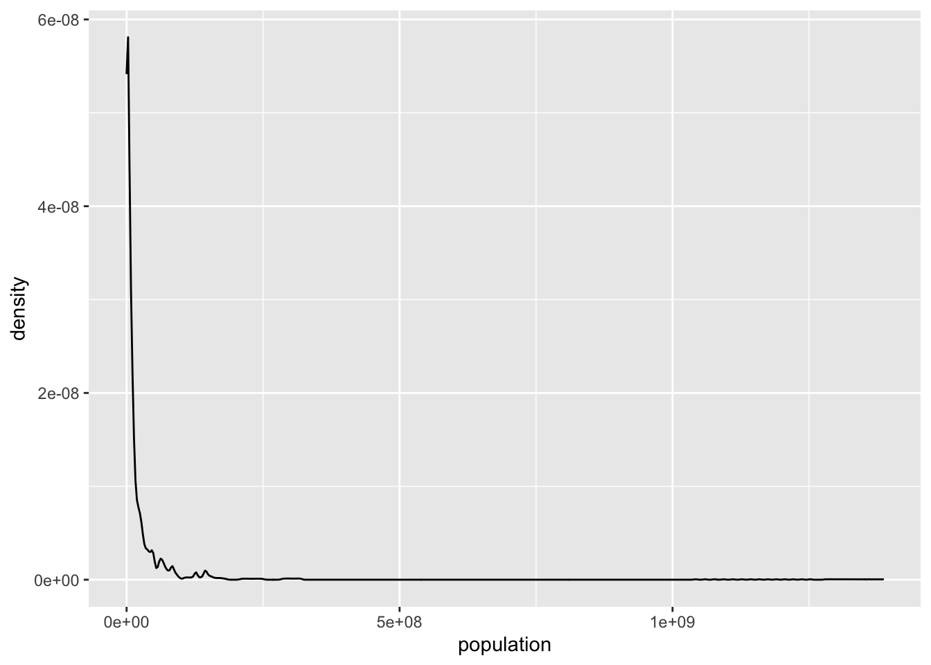
Figure 1.3: Population distribution
In a distribution plot, the y-axis shows the density and as a result it is calculated directly from the `
gf_density()function. As a result, we do not need to define \(y\) insidegf_density().
The population distribution is highly skewed: most countries have low population numbers, but very few countries have very high population numbers (100s of millions or even more than a billion). This concentrates the plot in te left side and creates a very long tail. These types of distributions are broadly described as power-law distributions. Their means are not informative, as they are being stretched by the very high scores of very few points. Their standard deviation is large, often higher than their means. For instance, in our example we see that the mean population is \(>30M\), even though the vast majority of the countries have lower population numbers (the \(75^{th}\) percentile population number is \(19M\)):
summary(tf)## country year population
## Length:2986 Min. :2000 Min. :1.129e+03
## Class :character 1st Qu.:2003 1st Qu.:6.202e+05
## Mode :character Median :2007 Median :5.398e+06
## Mean :2007 Mean :3.012e+07
## 3rd Qu.:2010 3rd Qu.:1.909e+07
## Max. :2013 Max. :1.386e+09The standard deviation, which we can estimate from function sd() is \(124M\), greater than the mean of \(30M\):
sd(tf$population)## [1] 123915350In fact, we can test it as follows:
sd(tf$population) > mean(tf$population)## [1] TRUE$ to isolate the population column from the tibble tf. This is one way of accessing a single column from a tibble. As a single column, population is perceived as a vector from functions sd() and mean().
In such cases, log-transforming the variable often results in more “normal-like” distributions:
#Let's log-transform this power-law looking distribution:
ggplot(tf, aes(x=log(population)))+geom_density()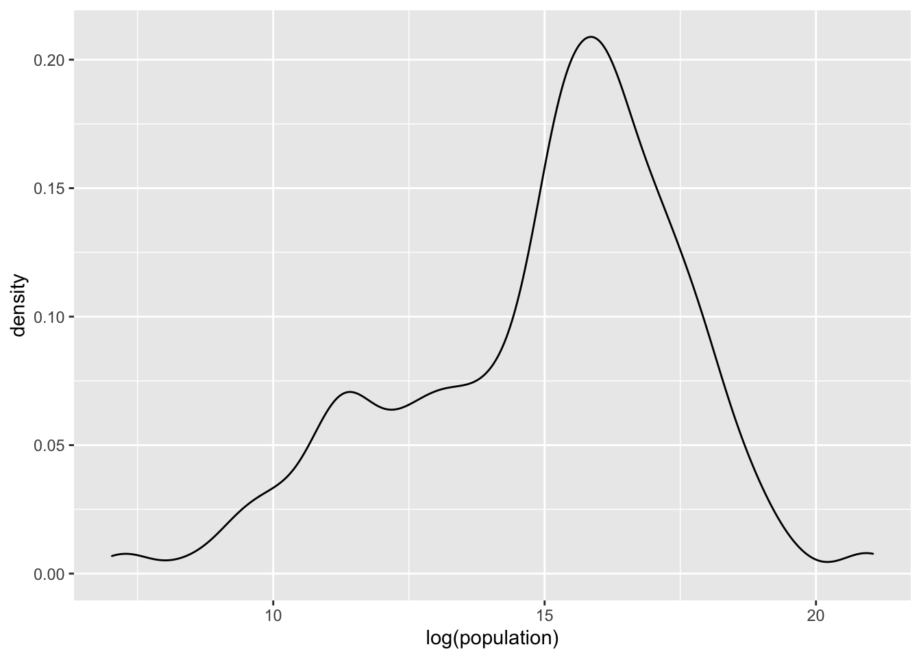
Figure 1.4: Log-transformed population distribution
ggplot2() in Section 3.
For comments, suggestions, errors, and typos, please email me at: kokkodis@bc.edu