7 Example: NBA data analysis
In this chapter we will scrape and analyze NBA data from basketball-reference.com. In this example, we will go over the majority of R functions that we have learned so far, and we will introduce a few new ones that can be particularly useful. Before running the code, check out the focal webpage: https://www.basketball-reference.com/
To start, load the following packages:
library(rvest)
library(tidyverse)
library(ggplot2)
library(ggthemes)
library(lubridate)
pluck = purrr::pluck
pluck = purrr::pluck is optional; it allows you to
call the function pluck without the purrr:: in front of it.
7.1 Scrape basketball-reference.com
Let’s first use read_html function to download the webpage that stores all the LA Lakers’ games from 2020:
r = read_html("https://www.basketball-reference.com/teams/LAL/2020_games.html")
r
## {html_document}
## <html data-version="klecko-" data-root="/home/bbr/build" itemscope="" itemtype="https://schema.org/WebSite" lang="en" class="no-js">
## [1] <head>\n<meta http-equiv="Content-Type" content="text/html; charset=UTF-8 ...
## [2] <body class="bbr">\n<div id="wrap">\n \n <div id="header" role="banner" ...7.1.1 rvest::html_table()
Because in this example we are interested in the available statistics, we will need to extract information out of the tables that are posted on the focal webpage. Instead of using the SelectorGadget extension, the rvest package has the function html_table that along with HTML tag “table” allows us to extract all the tables from a webpage:
r1 = r %>% html_nodes("table") %>% html_table() 7.1.2 purrr::pluck
This is great, but html_table returns all the available tables within an html web page. What if we wanted a specific table? Luckily, the package purrr that is included in tidyverse has a function called pluck that allows us to access elements from an R object through their index. For instance:
c(1,4,9) %>% purrr::pluck(3)## [1] 9
pluck I used the name of the package before the function, separated by two consecutive colons, to make sure that I am calling the pluck function from the purrr package. This is important to do because the rvest package has its own pluck function that works a bit differently and it might generate errors in our examples. So because both pluck functions are available in my environment, I need to specify which one of the two I want to use.
(In fact, in my case, because I have used
pluck=purrr::pluckin the very begining, I do not really have to use purrr:: front of pluck. I am only using it in case you copy-paste this code.)
Back to our example, let us assume that we want to get the second table; We can use the pluck function as follows:
r %>% html_nodes("table") %>% purrr::pluck(2) %>% html_table() %>%
  head
## # A tibble: 6 × 15
## G Date `Start (ET)` `` `` `` Opponent `` `` Tm Opp
## <chr> <chr> <chr> <lgl> <chr> <chr> <chr> <chr> <lgl> <chr> <chr>
## 1 1 Tue, A… 9:00p NA "Box… "" Portland… "L" NA 93 100
## 2 2 Thu, A… 9:00p NA "Box… "" Portland… "W" NA 111 88
## 3 3 Sat, A… 8:30p NA "Box… "@" Portland… "W" NA 116 108
## 4 4 Mon, A… 9:00p NA "Box… "@" Portland… "W" NA 135 115
## 5 5 Sat, A… 9:00p NA "Box… "" Portland… "W" NA 131 122
## 6 G Date Start (ET) NA "" "" Opponent "" NA Tm Opp
## # … with 4 more variables: W <chr>, L <chr>, Streak <chr>, Notes <chr>7.1.3 dplyr:bind_rows
If you notice, the two tables of the basketball-reference webapge store similar information; the only difference is that the bottom table stores information about the playoff season, while the top one stores information about the regular season. We can combine the two with the function bind_rows(). This function is similar to bind_columns, but instead of placing two tibbles next to each other, it concatenates one below the other:
r1 = r %>% html_nodes("table") %>% html_table() %>% bind_rows()The two tables have some non-matching columns, while the tables also include columns that do not have useful information for our analysis.
To get a list of all the available columns we can use the function names():
names(r1)## [1] "G" "Date" "Start (ET)" "...4" "...5"
## [6] "...6" "Opponent" "...8" "...9" "Tm"
## [11] "Opp" "W" "L" "Streak" "Notes"7.1.4 Drop, rename, and create columns
Now we can choose the columns we are interested in and rename them accordingly:
r2 = r1 %>% select(Date, Opponent, Tm, Opp, W, L) %>%
  rename(PointsFor = Tm, PointsAgainst = Opp, TotalWins = W, TotalLosses = L) %>%
  mutate(FocalTeam = "LAL")
r2 %>% select(Date, Opponent, FocalTeam) %>% head
## # A tibble: 6 × 3
## Date Opponent FocalTeam
## <chr> <chr> <chr>
## 1 Tue, Oct 22, 2019 Los Angeles Clippers LAL
## 2 Fri, Oct 25, 2019 Utah Jazz LAL
## 3 Sun, Oct 27, 2019 Charlotte Hornets LAL
## 4 Tue, Oct 29, 2019 Memphis Grizzlies LAL
## 5 Fri, Nov 1, 2019 Dallas Mavericks LAL
## 6 Sun, Nov 3, 2019 San Antonio Spurs LAL7.2 Custom functions and repetitive scraping
Our goal is not to just analyze the LA Lakers, but instead, to compare the performance of multiple teams.
Hence, it would be useful to create a custom function that extracts the above tibble r2 for any team we care about.
Then, we would be able to call that function repeatedly for different teams:
getTeamSeason = function(team){
  r = read_html(paste("https://www.basketball-reference.com/teams/", team,"/2020_games.html", sep=""))
  r1 = r %>% html_nodes("table") %>%  html_table() %>% bind_rows()
  r1 %>% select(Date, Opponent, Tm, Opp, W, L) %>%
    rename(PointsFor = Tm, PointsAgainst = Opp,TotalWins = W, TotalLosses = L) %>%
    mutate(FocalTeam = team)

}
Note that even though we did not use the return() function in the previous function, R by default returns the last estimated expression inside the function. So in this case, it will return the desired tibble.
Now we can call this function for any team we care about:
d1 = getTeamSeason("MIA") %>% select(Date, Opponent, FocalTeam) %>% headOr for multiple teams with the function map_dfr:
d = c("BOS","DEN","MIA","LAL") %>% map_dfr(getTeamSeason)
d %>% select(Date, Opponent, FocalTeam) %>% head
## # A tibble: 6 × 3
## Date Opponent FocalTeam
## <chr> <chr> <chr>
## 1 Wed, Oct 23, 2019 Philadelphia 76ers BOS
## 2 Fri, Oct 25, 2019 Toronto Raptors BOS
## 3 Sat, Oct 26, 2019 New York Knicks BOS
## 4 Wed, Oct 30, 2019 Milwaukee Bucks BOS
## 5 Fri, Nov 1, 2019 New York Knicks BOS
## 6 Tue, Nov 5, 2019 Cleveland Cavaliers BOS7.3 Transforming and creating new columns
7.3.1 dplyr::across
Many of the columns of our final tibble d are of type character, while they actually need to be numerical.
One way to transform these variables to numeric is to use the as.numeric function for each single one of them. However, we can also use the function across inside the mutate function which allows us to apply a third function on multiple columns:
#one by one:
#d$PointsFor = as.numeric(d$PointsFor)
#or all at the same time:
d = d %>%  mutate(across(c(PointsFor,PointsAgainst,TotalWins,TotalLosses),as.numeric))
7.3.2 Missing values
Let’s summarize our dataset to get a better idea of the ranges of each variable:
d %>% summary## Date Opponent PointsFor PointsAgainst
## Length:389 Length:389 Min. : 80 Min. : 76.0
## Class :character Class :character 1st Qu.:104 1st Qu.:100.0
## Mode :character Mode :character Median :112 Median :107.0
## Mean :112 Mean :108.1
## 3rd Qu.:119 3rd Qu.:115.0
## Max. :149 Max. :139.0
## NA's :22 NA's :22
## TotalWins TotalLosses FocalTeam
## Min. : 0.00 Min. : 0.000 Length:389
## 1st Qu.: 9.00 1st Qu.: 3.000 Class :character
## Median :20.00 Median : 7.000 Mode :character
## Mean :22.06 Mean : 8.981
## 3rd Qu.:35.00 3rd Qu.:14.000
## Max. :52.00 Max. :29.000
## NA's :22 NA's :22Multiple columns have missing values. Lets see why:
d %>% filter(is.na(PointsFor)) %>% select(Date, Opponent, FocalTeam) %>% head## # A tibble: 6 × 3
## Date Opponent FocalTeam
## <chr> <chr> <chr>
## 1 Date Opponent BOS
## 2 Date Opponent BOS
## 3 Date Opponent BOS
## 4 Date Opponent BOS
## 5 Date Opponent BOS
## 6 Date Opponent DENAs we can see, we have collected multiple unnecessary column names, along with a couple of games that did not happen yet. So we can mindfully remove these rows for the rest of our analysis:
d = d %>% filter(!is.na(PointsFor))7.3.3 Creating new columns
Let’s assume that we want to investigate whether the margin of victory of each game is an important statistic. First, we need to create a column that stores the difference in points that each team has won or lost:
d = d %>% mutate(WinBy = PointsFor - PointsAgainst)
d %>% select(Date, Opponent, FocalTeam, WinBy) %>% head
## # A tibble: 6 × 4
## Date Opponent FocalTeam WinBy
## <chr> <chr> <chr> <dbl>
## 1 Wed, Oct 23, 2019 Philadelphia 76ers BOS -14
## 2 Fri, Oct 25, 2019 Toronto Raptors BOS 6
## 3 Sat, Oct 26, 2019 New York Knicks BOS 23
## 4 Wed, Oct 30, 2019 Milwaukee Bucks BOS 11
## 5 Fri, Nov 1, 2019 New York Knicks BOS 2
## 6 Tue, Nov 5, 2019 Cleveland Cavaliers BOS 6Let’s get a quick average and standard deviation estimate for each one of the four teams:
d %>% group_by(FocalTeam) %>% summarise(mean(WinBy), sd(WinBy))## # A tibble: 4 × 3
## FocalTeam `mean(WinBy)` `sd(WinBy)`
## <chr> <dbl> <dbl>
## 1 BOS 6.06 11.8
## 2 DEN 1.21 12.5
## 3 LAL 6.03 12.9
## 4 MIA 2.73 12.17.4 Plotting with ggplot2
7.4.1 ggplot2::facet_wrap
Now let’s plot the distributions of the margin of victory for the four teams. The function facet_wrap allows us to visualize the distribution of each team in a separate plot next to each other. The functions scale_fill_brewer and scale_color_brewer allows us to use predetermined color palettes. You can find these palettes here: https://rdrr.io/cran/RColorBrewer/man/ColorBrewer.html
myPalette = "PuOr"
ggplot(d, aes(x=WinBy, color = FocalTeam, fill = FocalTeam))+
  geom_density(alpha=0.7, size=2)+facet_wrap(~FocalTeam, ncol = 2)+
  scale_fill_brewer(palette = myPalette)+
  scale_color_brewer(palette = myPalette)+
  theme_fivethirtyeight()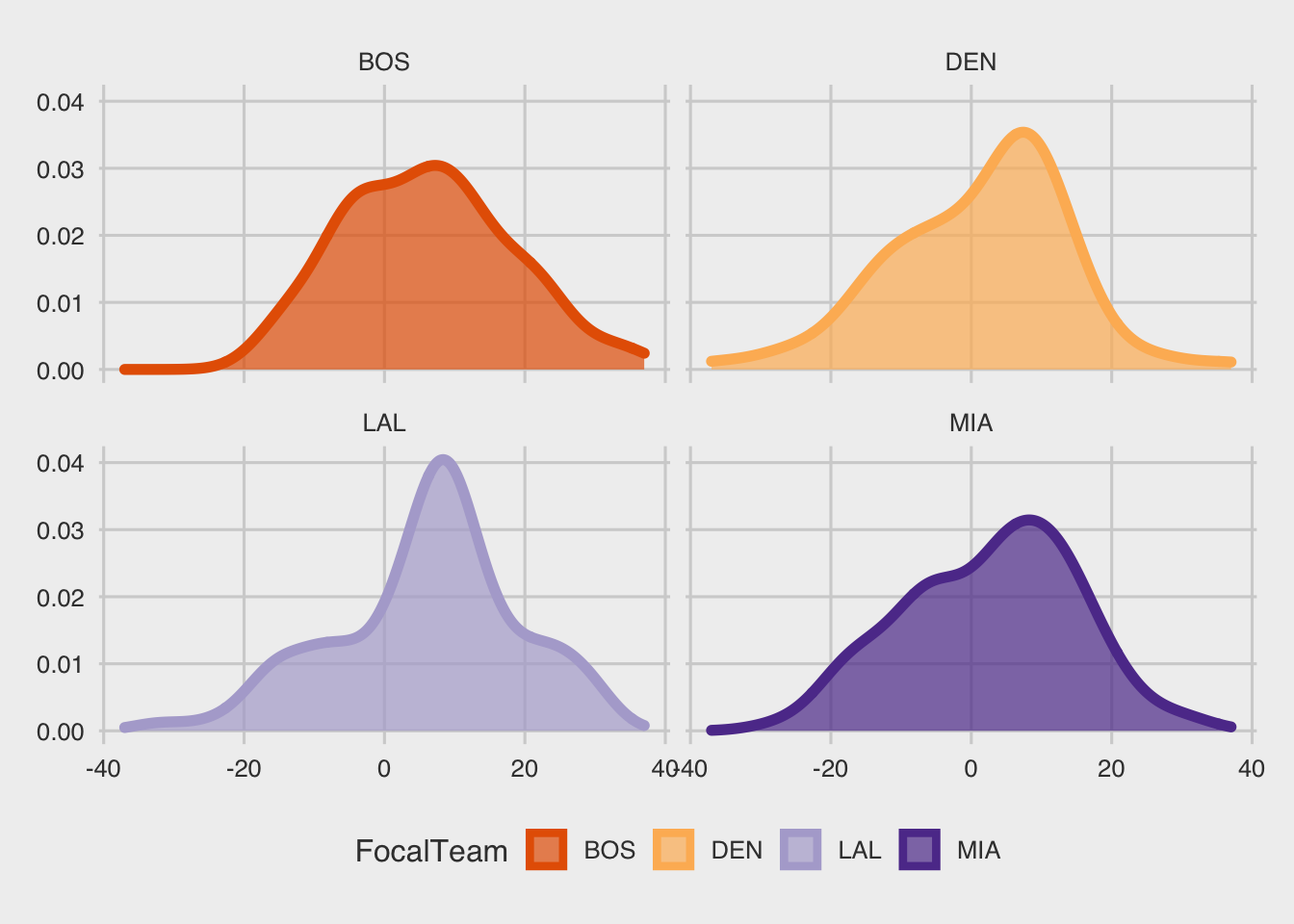
7.4.2 lubridate::as_date(,format)
If we look at our dataset we will see that the date column has a format that is not recognized as a date format by R. It would have been nice to be able to transform this format into an actual date type. Fortunately, we can do this with the function as_date that we have used in the past, along with its parameter format that we can set to match any specific date format:
as_date("Wed, Oct 23, 2019", format="%a, %b %d, %Y")## [1] "2019-10-23"An explanation of the format keywords can be found here: https://rdrr.io/r/base/strptime.html
We can apply this format to the column date and transform it to date type:
d$Date = as_date(d$Date, format="%a, %b %d, %Y")
d %>% select(Date) %>% head
## # A tibble: 6 × 1
## Date
## <date>
## 1 2019-10-23
## 2 2019-10-25
## 3 2019-10-26
## 4 2019-10-30
## 5 2019-11-01
## 6 2019-11-057.4.3 A linegraph
Now lets create a linegraph to see how the margin of victory evolved during the season for these teams:
ggplot(d, aes(x=Date, y=WinBy, color = FocalTeam, fill=FocalTeam))+
  geom_smooth()+
  scale_fill_brewer(palette = myPalette)+
  scale_color_brewer(palette = myPalette)+
  theme_fivethirtyeight()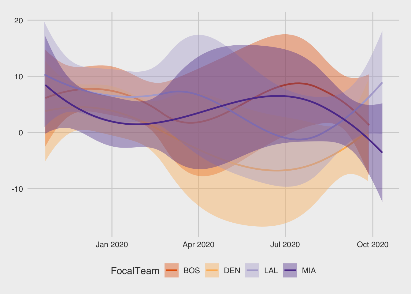
7.4.4 arrange(), head(), and tail()
We can rank the tibble so that we can see the top 2 victories (head) by margin, and the top 2 losses (tail):
d %>% arrange(desc(WinBy)) %>% select(Date, Opponent, FocalTeam, WinBy) %>% head(2) ## # A tibble: 2 × 4
## Date Opponent FocalTeam WinBy
## <date> <chr> <chr> <dbl>
## 1 2019-12-05 New York Knicks DEN 37
## 2 2020-01-11 New Orleans Pelicans BOS 35d %>% arrange(desc(WinBy)) %>% select(Date, Opponent, FocalTeam, WinBy) %>% tail(2) ## # A tibble: 2 × 4
## Date Opponent FocalTeam WinBy
## <date> <chr> <chr> <dbl>
## 1 2020-01-20 Boston Celtics LAL -32
## 2 2020-08-21 Utah Jazz DEN -377.5 Membership operator
Finally, let’s assume that we only want to save into a csv file information about Boston, LA and Miami, and ignore Denver. One way to do this, is to use multiple OR statements or just use FocalTeam != 'DEN' inside a filter function. Another way to do this, which sometimes is more useful and more intuitive, is to use the membership operator %in%. For instance, the following asks whether 5 is included in the vector c(4,6,7):
5 %in% c(4,6,7)## [1] FALSESimilarly, in our case, we can save this file as follows:
#LAL,BOS, MIA
write_csv(d %>% filter(FocalTeam %in% c("LAL","BOS","MIA")),
          "../data/nba.csv")
For comments, suggestions, errors, and typos, please email me at: kokkodis@bc.edu